Local Retrieval Augmented Generation (RAG) from Scratch (step by step tutorial)

Daniel Bourke builds a complete RAG pipeline on a local GPU from scratch. He loads an open-source LLM like Gemma 7B, embeds a 1,200-page nutrition textbook, retrieves relevant chunks for user queries, and generates answers. The tutorial covers quantization, prompt engineering, and wraps everything into a single function.
Chapters
Hello everyone, Daniel here. In this video tutorial, we're going to start from a blank notebook and end with a full Retrieval Augmented Generation pipeline, or RAG pipeline, from scratch. And best of all, it's going to run on our local machines, all to showcase the power of AI on RTX. Have a look at that GPU. NVIDIA have been so kind to send me an RTX 4090 GPU, so Shout out to Mark, thank you so much for that. Now what this means is that if you have a PC with an NVIDIA GPU, you've got a gym. No, no, I'm joking. It means you've got a machine that's incredibly capable of AI workflows. So I've got all the code here on GitHub. We're going to write this line by line together in this video. Check the link in the description for that. But it's also to celebrate the upcoming NVIDIA GTC conference, which is happening from March 18th to 21st. But if you've already— you're watching this in the future and it's already happened, there's a heap of sessions that are going to be virtual. So it's happening in San Jose, California. I live in Australia, so I'm going to be attending virtually. I've got 3 sessions lined up that I'm looking forward to. This is Retrieval Augmented Generation, an overview of design systems. So this is similar to the pipeline that we're going to be building in this video. There's some NVIDIA software in here, TensorRT LLM. Uh, we don't explicitly cover that, but that's what I want to learn more, potentially for a future video. So let me know if you want to see that. And then I also have saving trees in forests all over the world using AI, a really cool application, uh, to identify 600 different species of trees on a mobile phone with a macro lens. That's so cool to me. And then we have here building a deep learning foundation model via self-supervised learning, which is a really powerful technique that what large language models use to learn. They use self-supervised learning to learn from large corpuses of text, but this is bringing it to computer vision. So once again, all the code's on GitHub, the links will be in the description. Follow along if you'd like to build your own very own RAG pipeline from scratch running on your own PC. I might have to move this to the floor because it is quite loud running here. If you have any questions, leave a discussion on the GitHub page or a comment below. And let's build. Hello, hello. Welcome to the simple local RAG tutorial. Now we're going to rebuild this workflow and we're going to have it run all locally on our own GPU. And if you want the materials for this, they're on the GitHub. So I'll put that link in the description. And if you want to run it in Google Colab, maybe you don't have a local GPU available. You can click on the link here. It's all in the GitHub. This same workflow that we're going to go through, uh, will all run in Google Colab. So let me just jump into what we're going to do. You can use this notebook here as a reference, but we're going to code this whole thing up from scratch. There's some information here. What is RAG? Why RAG? If you never heard it, you're going to be— we're going to be saying RAG a lot during this video. What kinds of problems can RAG be used for? Why local key terms? What we're going to build, all that sort of stuff, all the code and explanations are in this notebook. A lot of vector outputs there. So that's where all those numbers come from. They're from our embeddings, but we're going to get to that. I'm just giving you this so you can use it as a reference because we're going to code all of this up from scratch. So let's jump into an example workflow. And by the way, we're going to take this quite slow. We're going to write every line ourselves. Um, so if you have any questions or issues, leave a comment on the video or a discussion on GitHub or an issue if there's something wrong. If you want to get set up, all the instructions are here, but we're just going to go through this step by step. So what is RAG? Well, RAG stands for Retrieval Augmented Generation, and I've stolen this image or this flowchart from NVIDIA's blog. So they have a great blog post which is Demystifying RAG 101, and that's kind of what I've based this workflow off, except we're not using a framework. We're going to be writing all of it ourselves. We're not using Llama Index or LangChain, which are two great frameworks, and they can help to process these workflows, but we're going to see what it looks like just to do with, with Python and PyTorch and Transformers and whatnot. And then in that way, in the future, if you'd like to use LangChain or LlamaIndex, well then you know how to do it yourself. So that's sort of what we're going to be building. If you want to read more, the link to that is available. I'll link this little whiteboard that I'm using as well. But let's dive into it. So what are we going to build? Well, we're going to break it down into two major parts. The first part is document preprocessing and embedding creation. And the next part is search and answer. But before I jump into this flowchart, we might as well break down what RAG is. And so I've set up my computer to already go through the setup steps. So if you go to the GitHub, I've gone through these steps, git clone, and now I'm using Python 3.11 on a Windows 11 machine. With an NVIDIA, uh, RTX 4090. So that NVIDIA have so kindly given me to create this video in partnership. So there we go, um, there's an NVIDIA GeForce RTX, but this should work on almost any local NVIDIA GPU. So that, of course, the RTX 4090 at the time of recording is one of the best ones you can buy from a consumer level, but it should work on most modern NVIDIA GPUs, and we put some code in there. So if you've got an older GPU with less memory, it should still work, and we'll discuss that later on when we get into model usage. So I've gone through these setup steps, and that's what I've got here. Excuse me, I'm still getting used to Windows. Um, I've created an environment, I've activated it, I've installed the requirements. And if you run into any issues setting up the requirements, I put some notes here, but we can 2 things that we can do if we want to run locally. We can use VS Code. And so I can just type in code dot and that'll bring us up here. This is the same repo just running on my local computer. And then if you want to start a new notebook here, we can just go oosimple_local_rag and I'm going to call it.video IPython notebook. And then we can just start from here. Import torch. Shift and Enter, we'll select our Python environment. We can run it there. So import torch. So there we go. However, I personally have found, and maybe I'm doing something wrong because I'm not, I'm not used to using Windows, that VS Code kind of lags a little bit for me when I have a large notebook. Maybe I'm doing something wrong. If you know about this, please let me know. So what I'm going to do instead of pressing Code., I'm going to start with a Jupyter Notebook. So Jupyter Notebook. But the same process will run whether you're using a VS Code notebook, which should technically be the same as using Jupyter. So now I'm using a Jupyter server, which has the same files that my VS Code setup has. But I'm just going to use Jupyter. If you want to use VS Code, you can do that as well. So let's jump into this. Dismiss. Oh, what's going on here? Oh, oh, I haven't saved it here. Of course. That's an interesting error. See, I'm going to leave some of the errors in here, you know. So let's see if it opens up now that I've saved it. Okay, there we go. We get Torch. And I'm going to zoom in a little bit there. That should be good. Okay, so let's— I know that was a bit of an intro, but again, all I've done here is I've gone through the setup steps. I've just done this in the terminal, git clone, cd into simple_local_rag, created an environment, launched it, and then installed the requirements in that environment down here. If you'd like to see a dedicated setup video to this, please let me know and I can make one of those. but now I'm at this stage. I've just gone Jupyter Notebook and we are in like the kid in the tree. All right, so let's create a title for this. So we want to create and run a local RAG pipeline from scratch. Now of course it won't be 100% from scratch, uh, we won't be training any embedding or LLM models here, but we will be using them. So let's define what is RAG. What is RAG? So RAG stands for Retrieval Augmented Generation. You may have been seeing this quite regularly in the world of LLMs and generative AI. Essentially, the goal of RAG is to take information and pass it to an LLM so it can generate outputs based on that information. Now, that's a pretty broad statement, but that's on purpose because RAG can really be that broad. Oh, let me turn this into markdown, escape an M, by the way. So that's what we want to do. We have information in one place and we want to pass it to an LLM so it can generate information. Now, why would— based on that information that we pass it, That, that could be the prompt. So let's break each of these steps down. So we want retrieval. So retrieval is another word for search. So find relevant information given a query. E.g., in this project, we're going to be building NutriChat, which is chat with a PDF. Now we'll break this down a bit more, but we have a nutrition textbook that's 1,200 pages long and we want to chat with that textbook. So we might ask a question of what are the macronutrients and what do they do? So e.g., what are the macronutrients and what do they do? Right? So find relevant information. So we'll turn that into retrieves passages of text related to the macronutrients from a textbook, a nutrition textbook, by the way. And then we have augmentation or augmented. So augmented is we want to take the relevant information to take the relevant information that we got from retrieval and augment our input prompt. So often the input to an LLM is called a prompt. Our input prompt to an LLM with that relevant information. Now we'll discuss why we want to do that in a second. And then we have generation. So take the first two steps and pass them to an LLM for generative outputs. Beautiful. So retrieval augmented generation. So if you've ever used an LLM, ChatGPT is a great example. So what are the macronutrients? And what do they do? So this is a sense— this is not actually using retrieval augmented generation. This is, as far as I know, ChatGPT is just generating this based off what it's learned in its training data. So why— this is still helpful, but why might we want to use retrieval and then augment our prompt? So this is my prompt here. Why might we want to augment that with relevant information. So let's discuss why RAG. Why RAG? So the main goal of RAG is to improve the generation outputs of LLMs. So if we go back to ChatGPT, we got a pretty good output here. Now, I've studied nutrition And I would say this is a pretty good high-level answer. Macronutrients are the nutrition— nutrients that our bodies need in large amounts to function correctly. They can be divided into 3 main categories: carbohydrates, proteins, and fats. And then we've got a little breakdown. So that's a, that's a good answer there, right? However, this is quite a general question. You might find a lot of information on this on the internet, and that's what most large language models are trained on. They're trained on internet corpuses of text. So terabytes of text data. However, what if you have private information, or what if you have factual information that an LLM won't have access to? That's where RAG can come in. So number 1 would be to prevent hallucinations. So let's say, um, LLMs are incredibly good at generating, um, good-looking text. However, this text doesn't mean that it's factual. Right? So let's say you're a business and you have a customer support page. Let's go to ChatGPT. My— so Telstra, is a telephone company in Australia. So let me just go to Telstra, Telstra customer support. And I know this is an actual project because one of my friends is working on this. So call us, message us. Where's search? So say I wanted to search Telstra. So this is a phone provider in Australia. So I want to search My bill was too much last month. Right. That's very natural language there. But what if we could get— see, this website is giving me grief. What if we could get an answer rather than just this list of links here? Make a complaint. Do I want to make a complaint? Hmm. I'm not sure what's going on here. Anyway, we get a lot of support documents. So what if you're, what if you're Telstra or any other company that has a lot of customer support problems? And I asked ChatGPT the same question. So my Telstra bill was too much last month. If your Telstra bill was unexpectedly high last month, there are several ways you can do it. Review your bill. So this is going to be generic information, right? But what if we had a ChatGPT that was linked, or a similar language model, because ChatGPT after all is a large language model, that was linked with all of Telstra's customer support documents, and we could talk to it when we have a problem. So see how this is just like generic information. That's what you expect with anything. But we want a specific— we've got a specific problem. We want our question to be answered with Telstra's customer support. So that is where RAG can come in handy, is what you would do in this case is, for example— now this is not necessarily a hallucination, or actually let's go to the number 2 hallucination. Um, RAG can help LLMs generate information based on relevant Passages that are factual. So there we go. We've got number 1. Now, number 2 is what I just talked about. So hallucinations is all of this text looks good, but it doesn't necessarily promise you that it's going to be correct, if that makes sense. It could look good and read well, but it doesn't mean it's factually accurate. So that's what we want to do with number 1 with RAG is we want to provide our LLMs with factual information, so information that we have stored somewhere, and then we want to go, hey, can you process this information to answer my query? And then number 2 is work with custom data, right? So many base LLMs are trained with internet-scale data. This means they have a fairly good understanding of language in general, right? So if I ask a query of ChatGPT, I've got a problem with my Telstra bill, it's going to give me some pretty good answers, but it's not Telstra-specific. Whereas I typed this into Telstra's website, in an ideal world, they take all their customer support documents and put it into a system, a RAG pipeline, and then I would get an answer back in similar style to ChatGPT, but based on Telstra's actual documents. That's the whole premise of RAG, is to use your actual documents and process them and deliver them in a generative way. So retrieval, find the relevant Telstra documents that are related to my problem. Augmentation would be to— my bill was too much last month. That's my query there. So augmentation would be to take passages from these documents put them into my query here, and then have generation— an LLM like ChatGPT would be to take those documents and return them or options for me in a legible, readable way. That's the whole premise of RAG. So, and of course, there's many more aspects to this, but this is, this is an actual problem that one of my friends in Australia works with quite a large tech company. Is helping Telstra to work on right now. So that's just a concept of where RAG gets used in the workplace. So this means they have a fairly good understanding of language in general. However, it also does mean a lot of their responses can be generic in nature. So RAG helps to create specific responses based on specific documents, e.g., your own company's customer support documents. And I want you to start thinking about documents as being a very broad term. So documents could mean just like thousands of PDFs, hundreds of customer support documents, heaps of text files, your emails. Let's get into some use cases, right? So we've already discussed one. So what we want to do is what can RAG be used for? So that's one very helpful use case. We've all been to a customer support website and just had absolutely no fun trying to get some help like I just had here. The Yeah, won't even let me type anymore. Okay, so Telstra, I love you, but you're an Australian company and you need a little bit of help on your search options here. So let's go, what can RAG help for? So number 1 would be customer support Q&A chat. So treat your existing customer support documents as a resource. And when a customer asks a question, you could have a retrieval system. We're going to build this later on, don't you worry. Retrieve, retrieve relevant documentation snippets So pieces of text from the documentation rather than— can you imagine having to go through what's an order estimate? It's an estimate of how much your first bill, your monthly charge after that. No, this doesn't help. My bill is too much. Why have I received a final bill? Get help on your bills and payments. Okay, see, look, I just want to— just give me the answer. There's too many options here. Okay, I'm not ditching on Telstra. This is a lot for a lot of companies. This is a big problem, right? Customer support is a very hard thing to do. So retrieve relevant documentation snippets and then have an LLM craft those snippets into an answer. And so you can think of this as a chatbot for your documentation. Now, I know there's been a lot of chatbots in the past, but over the last couple of years, chatbots have actually got really good. So this is no longer so much of a gimmick. It actually really works. For example, Klarna LLM customer support. Here we go. So this is a big example. Klarna is quite a big financial company. So let's go Klarna market cap. So Klarna raised— yeah, there you go. Worth multiple billions of dollars apparently. So quite a big company. And has used AI assistant to handle two-thirds of customer service chats in its first month. So big details here. Yeah, there we go. So AI has handled 2.3 million conversations. So this is where RAG pipelines can help out. So you type a message to Klarna, it goes through its customer support documents. I've got this problem. And then it gives you an answer. And it's based on— is it OpenAI? Yeah, based on OpenAI. So this is the exact workflow that I was just talking about. We have a ChatGPT like model plugged into our own documentation, right? So we go back to Klarna and they strive $40 million US in profit in 2024. That's incredible. So let's keep going with our use case. We want to learn how to build these systems, right? Then we have another option, which would be email chain analysis. So there's plenty of options here. So this is another thing, project that my friend is working on. Let's say you're a large insurance company. And you have chains and chains of emails of customer claims, right? So you could search through all of those emails by hand, and that would take quite a long time. So you could use a RAG pipeline to find relevant information from those email chains and then use an LLM to process that information into structured data. So basically take the unstructured text and turn it into something like JSON or something structured or a spreadsheet or something like that, right? And then we have another one which could be company internal Documentation chat. That's quite similar to the customer support Q&A. But if you're a large company and you have an internal documentation set or even your own computer, I'm still getting used to using Windows, but I'm quite used to using my Mac. I'd really love it if the assistant on my Mac— I'm not going to say it out loud because it might trigger somewhere in the house, but it starts with an S and ends in -ery— could search all of my documentation via just chat instead of me having to use keywords. And then we have another one, which is what we're going to build— textbook Q&A. So let's say, let's say you're a nutrition student. And you've got a 1,200-page textbook to read. You could build a RAG pipeline to go through the textbook and find relevant passages to the questions you have. So the premise here is all the same. So retrieval augmented generation. I like to think of it with all of these use cases, the common theme, common theme here is take your relevant documents to a query and process them with an LLM, right? So from this angle, you can consider an LLM as a calculator for words. Quite a different concept here because in the last few years, LLMs have gotten very good at processing language in general. So RAG is from one angle— oh, Grammarly, goodness me, How do I turn that off? Grammarly is invading everywhere. Um, one second, I'm just going to turn off Grammarly. Excuse me for this. Uh, I don't know how to do that. Anyway, I'm going to ignore it, right? So an LLM as a calculator for words. Now one more point to go on is why would we want to run this locally? What if ChatGPT is already good? Well, locally is like you got your own car, right? You like to drive that. So that's what I imagine is why would you want to run these, these systems locally is, well, it's fun to drive your own car. First of all, fun. So fun to build your own pipelines and software and run it locally. And then of course you've got the practical benefits, which are privacy, speed, and cost. So privacy, if you're a big company, with private information. So if you have private documentation, maybe you don't want to send that to an API, right? Maybe you don't want to send your information to OpenAI or Anthropic with Claude or Google or whatnot. So you want to set up an LLM and run it on your own hardware. And then number 2 is speed. So, um, whenever you use an API, you have to send some kind of data across the internet. This takes time. So you'll notice with ChatGPT is That answer didn't quite help. Can you search Telstra's customer support documentation for me? Let's see if it can do that. Does it have a web browser? Maybe it does. But see, this time we have to wait for this to happen. So maybe it's 5 seconds. There we go. It's pretty quick. Yeah, see, we're not getting— or maybe it did search. Oh, there we go. Okay, that's pretty good. But we still have to wait for time for that, right? So locally is— running locally means we don't have to wait for transfers of data. So we don't— our data doesn't have to go off onto the internet. It can run on a local machine that I'm running under my desk on this particular GPU. So NVIDIA SMI, it's going to run right there on that hardware, so it's going to go quite quick. And then 3, of course, is cost. Now there's more arguments here, but these are the 3 big ones that I've picked out. Of course, fun— you like to drive your own car around the place, you don't always like to just hire a car and drive it. So cost is if you own your hardware, the cost is paid, right? So buying new hardware may have a cost. It may have a large cost to begin with, but over time you don't have to keep paying API fees. And then probably another important one actually here is no vendor lock-in if you run your own software/hardware. So for example, if I rely on ChatGPT to run my business, if OpenAI/another large internet company shutdown, if they shut down tomorrow, you can still run your business. Right? I don't think OpenAI will shut down tomorrow. But this is just, I mean, you've got your own hardware and software, you're running that, it doesn't matter if they shut down tomorrow. So these are, these are 4 really big points. So that's about enough for the intro of what is RAG, why RAG, what RAG can be used for, and why local. Now let's start to just dive into the project that we're going to do. So I'll just pause the video here. I'm just going to write pause for myself when I edit this and I'll come back in about a couple of minutes. But if you want to take a little break and come back, we're going to start going over the project we're going to build and we'll write some code. Okay, I'm back. So we just talked about what is RAG, why RAG, what can RAG be used for, and why local. Now let's jump into— I'm just going to— maybe I'll leave a link here, or let's discuss what we're going to build, actually what we're going to build. Now I've got two resources. We've got simple_local_rag, that's the GitHub. I'm going to put this in here, one, and then this, I'll share that as well. Copied link. Beautiful. This is a little nice little whiteboard that I've got. So I'm going to put that there as well in case you want. These will all be in the description as well. Let me just close. So we don't need— we'll keep those just in case. So the reference here is for all the code, by the way. Now I've skipped one thing. I haven't gone over the key terms, but if you want to read those, you can do them here. I'm just going to explain them as we go. We've got token embedding, embedding model, similarity search, vector search, large language model, LLM context windows. Sorry, I'm talking too fast. Prompt. Now there's some key terms to read, but we'll go through them as we go. Right. Notebook. Beautiful. So let's just jump into here what we're going to build. I want my little workflow document. There we go. So let me zoom in. We have 2 major parts here: document preprocessing and embedding creation, and then search and answer. I'm going to break these down, and it's all going to happen on a local NVIDIA RTX 4090. So let's say you have a dataset of documents. Now, again, documents is very broad. I just say a large database of PDFs. It could be a large database of customer support articles. It could be internal documentation. It could be email chains. It could be almost anything to do with text. And now we're starting to get into the realm of images as well, but we're going to focus on text. I have a 1,200-page nutrition textbook, and if I go to this link in the GitHub, it's an open-source textbook, but this would work with almost any textbook. Human nutrition. I love food. I love nutrition. I'd love to learn more about it. So frankly, I'm building this system for myself. We could do all of the nutrition articles on Wikipedia as well, but we're just going to start with a PDF to begin. So I've downloaded it here, digital PDF. And I've included it there, Human Nutrition Text. I've renamed it. It's open source, so you can check it out. It might be a bit too big to load in the browser though. Anyway, that's our PDF. Can I download this? Yeah, there we go. Let's have a look at it. Human Nutrition Text. We'll open it up. We've got heaps of pages here. So we could search through this. So there's the people who have authored it. Let's just scroll right to the bottom. How many pages do we have? A lot of pages. I might just take this. This is taking a bit too long. So 1,200 pages. Of course, a lot of them aren't— they're on— aren't all text. A lot of them are just reference and whatnot. But what if we were to search for What are the macro— okay, we've already— it's not there. We can't do a general query like that. We can do keyword matching. Macronutrients. There we go. So what if I, instead of searching just like this, I could chat with this document? That's what we're going to build. So what we have to do is we take that PDF and then we preprocess that. We're going to write code for all of this. We preprocess the text into smaller chunks. So rather than it— I'm just gonna X out of this— rather than it being— the text in here is actually pretty big on these pages. I'll just zoom into that as well. Rather than it being a full page, we might break this into something like 10 sentences. And I know that because I've already tried and I've already made the material. So I know how many sentences we're gonna break it into. But this is still an active area of research in how to chunkify or make your text smaller. Then we have smaller documents. So these are going to be our context, our retrieval passages that we're going to pass to our LLM later on. And so what we do is we embed these smaller chunks of text. Now, what I mean by that is embedding is a numerical representation that makes data useful. That's all we have to know for now. We're going to see what it looks like hands-on. And then we store these somewhere. We could store them in PyTorch tensor. If you're not familiar with PyTorch, I have a great video on PyTorch. You might want to check that out. And we could also store it in a database so that we could use it later. And then we come to the next step. So that's one step, embedding creation and storage. Now we have search and answer. Now that starts with a cool person. Maybe this is you. I quite love— let me just show you something. If you search for person, there's two people here with sunglasses on. They're like in business attire. They look like, like a spy movie or something like that. But yeah, so cool person. Maybe that's you. You ask a query of your information here. What are the macronutrients and what do they do? Now what we do is we embed that query with the same model that we embedded our documents with. Now again, in embedding, we just have to think of it as a numerical representation because computers don't deal with text as well as we do. It might appear that they do with ChatGPT, But behind the scenes, ChatGPT is— when I ask a question, so how much does an elephant weigh? It's going to turn that query into a numerical representation and then it's going to quiz its weights of which are also numbers of go, hey, have you seen the numbers from this? Show me other numbers that are similar to that of what a response would look like. So computers deal with numbers even though this appears as text behind the scenes. And we're going to, we're going to do this ourselves. We're going to turn words into numbers. And back again. So we embed our query, and this is important, with the same embedding model that we used to embed our documentation. And then we can store that embedding, uh, query if we wanted, so we could cache it later. But usually it's quite quick just to embed it once at a time and search. And then what we do is we find— this is the retrieval part of Retrieval Augmented Generation, or RAG— we find similar embeddings So these will be numerical representations that match our query. I'll show you how to do that later on. We're going to write code to do so. And then this is the augmentation part, is we take our question here. I know that's a bit small, but we take our question here, we append the relevant passages from our text, and we pass this to an LLM. So imagine if we're talking to ChatGPT and we've got, um, My Telstra bill is too much. But then we have context item 1 and then context item 2. Oh, right. And then, sorry, I'll go context item— I got a bit trigger happy there. And then we go, please create an answer to the problem based on the context. So there's context item 1, 2, 3, and these could be 3 articles that are relevant somewhere. I'm not even sure where I went. Check your account details. There we go. So an article like this, again, this is just an example. It's not the right article, but an article like this that is related to my problem. And we could put another one there and another one there. And then we ask our Calculator for Words to create an answer to the problem based on these three contexts rather than just creating a bit of a generic answer here, right? So that's what we're going to do there. And then this answer comes back to us along with the resources. Now, this is an important point. We can get the answer, but as well as where the answer came from. So then we can go and verify if that answer is actually correct. So in the case of nutrition textbook, we could ask, What are the macronutrients and what do they do? And our LLM could return us a response. But not only that, but go, hey, this is where I got the information from. I got it from page 5, macronutrients. And then maybe it found another page somewhere later on. I'm making this up. And it said, this is pretty helpful as well. And it's like, this one's also pretty helpful if you want to learn more, wherever it is here. Okay, that's just an example. I'm not— these aren't specifically related. I'm just saying that that's the type of system that we could build. Not only are we getting the answer, we're also getting resources to that. And so you can imagine how helpful that is for a customer support system, is you get an answer, but it's like, hey, read this documentation for more. Or if you're in a large company and you're like, what do I do when I need to lodge an invoice? And the response says, hey, you can lodge an invoice by here. And this is what you do. This is our process. All that sort of jazz. But with that being said, we've got our beautiful little diagram here. We're going to be coming back to this quite often. But let's just write some steps. So we're going to build— I'm calling the project NutriChat to chat with a textbook, nutrition textbook. But again, I want you to keep your mind open to the fact that textbook here could be anything, a collection of PDFs, a collection of text documents, a collection of customer support documents. Really keep your mind open to this because we're only— this is still quite a new workflow, RAG. We're only really scratching the surface of this. Oh, and I forgot one more thing up the top here while I've got it in my mind. If you want to read where RAG came from, See the paper from Facebook AI. So originated out of Facebook AI, a fantastic AI team. So if we search RAG paper, is this going to work? Oh, there we go. Google's pretty good. So Retrieval Augmented Generation for Knowledge-Intensive Tasks. So this is a machine learning paper. If you've never read one of these before, they can be quite intimidating, but essentially what we get to is this is a really technical way of describing what we've just described. They've got— I really love this last paragraph. So this is explaining what RAG is. So the work offers several positive societal benefits over previous work. The fact that it is more or less strongly grounded in real factual knowledge, in this case Wikipedia. So they— their example was they used a large language model GPT-2 maybe, and they generated outputs based on Wikipedia text. So it makes it hallucinate less with generations that are more factual. So hallucinate less, that's really important, and offers more control and interpretability. So you know where the generations came from. So RAG could be employed in a wide variety of scenarios with direct benefit to society. For example, by endowing it with a medical index. Oh, there we go. So you could give it like, um, all of, uh, medical journals and that sort of stuff, and asking it— or PubMed, that's what I was looking for— and asking it open domain questions on that topic, or by helping people be more effective at their jobs, right? So if you can get information quickly, you can work quickly, right? So let's put this in our notebook. So that's their conclusion there, and I'm just going to put this— it's a great paper to read, Retrieval Augmented Generation for knowledge-intensive NLP tasks. So you see, 12th of April 2021, so it's, it's barely— it's under 3 years ago that this paper was published, and RAG is taking over many different workflows. So we're going to learn how to build a system like this for ourselves. We go there. Wonderful. Now, so specifically, let's get into what we're going to code. Step 1, and I know we're going a bit all over the place, but that's all right. We're going, we're going slow here. We're going to write every line of code ourselves, and I want to try and explain it as much as I can. So you could use almost any PDF here, or even a collection of PDFs. 2, we're going to format the text of the PDF textbook. Ready for an embedding model. So we want to turn our text into numbers with the embedding model. So we're going to embed all of the chunks of text in the textbook and turn them into numerical representations, so an embedding, at which we can store for later. And I'm just going to put this as embedding. Oh my goodness, Grammarly. I'm going to get rid of that in the next break. I'll just make sure I'm nice and zoomed in there and then build a retrieval system that uses vector search. We're going to talk about what this is later on to find relevant— or if you're trigger happy, you can skip ahead and just go to all the code. Relevant chunks of text based on a query. Now vector search is one of my favorite techniques that I've ever learned in machine learning, so I'm really excited to share that with you. So create a prompt that incorporates the retrieved— this is basically just the text version of our nice image, right? Pieces of text. Incorporate— would help if I could spell, then Grammarly wouldn't be so much of a hindrance. So generate an answer to a query based on the passages of the textbook. With an LLM, all locally, all locally. So step— major step 1 is steps 1 to 3. We'll call this document preprocessing and embedding creation. And major workflow 2 is steps 4 to 6. We'll call this search and answer. All right, that's beautiful. So this is our— what we're going to build. Number 1, document processing and embedding creation, and number 2, search and answer. So with that being said, we can— I know I said we were going to start coding in the last section, but, uh, how about in the next section We start off number 1. We're going to go number 1, document/text processing and embedding creation. And I'm going to write a little note here for pause. So future Daniel, pause and let's take a break and I'll be back in a couple of minutes. And I'm back. Let's start Step number 1: document text processing and embedding creation. So let's treat this like a machine learning cooking show, hey? We need a couple of ingredients. Might just put this in the center of the page. There we go. Ingredients: we're going to need a PDF document of choice, and I want you to note here, note this could be almost any kind of document. I've just chosen to focus on PDFs for now. So keep your mind open. I'm going to sound like a broken record here too. RAG can work with— if you've got text, you can probably set up some sort of RAG pipeline there. So embedding model of choice. Now we're going to get into that in a second. So we need a PDF document and embedding model of choice. Won't necessarily have those ahead of time, but we're going to get that later on. And then the steps. So number 1, we want to import our PDF document. Number 2, what we're going to do is process text for embedding. So eg, split into chunks of sentences, right? Number 3 is embed text chunks with embedding model. And number 4 will be save embeddings to file for later use. So embeddings, in terms of a cooking show, embeddings will store on file for many years or until you lose your hard drive. In essence, they don't really have a best before date as long as you have access to the model that you embedded them with. Because yeah, if you have embeddings but not the embedding model, Finding a query on them anyway, that might be a bit hard. We'll find that on— we'll see that later on. So let's start with importing a PDF document. Now of course, like any good cooking show, I've prepared ahead of time. So import PDF document, but we want to do things for completeness here. You might not have the PDF that I have. So this is our PDF, and of course I downloaded it from here, the website. It's in Oh, sorry, it's on GitHub if you really want it. There we go. But how about if you're— you want to download it programmatically, which I like to do if you don't necessarily have access to it. So I'm going to start by importing— oh yes, we're finally writing some code. Uh, thank you for your patience if you've made it all the way to here, but I promise you the rest of the video will mostly be code. Now, um, let's get our PDF document. Get PDF document. Path. So PDF path equals— now we're only working with one PDF, um, so if you're working with a folder of PDFs, you could alter the code a little bit for that. But this is a 1,200-page PDF, it's quite a large one. So we already have the file, just keep in mind, but I'm writing some code here to— so if we didn't have the file, we can get it. So let's download— by the way, OS is Python. For os module, and request is going to help us download things off the internet. So you can look up the documentation by this, python requests, and we got requests. Does Python documentation URL lib request? Anyway, let's see how it's used, right? And if you want to look up the methods, you can do that. So download PDF. So if the path doesn't exist, so if not os.path os is going to help us deal with our operating system. So we're going to look for this path, and if it doesn't exist, we want to download it. Okay, so pdf_path, and then I'm going to print a little info statement here. You'll find I like to do a lot of little prints, see what's happening. So file doesn't exist, downloading, right? And then we're going to go, um, enter the URL of the PDF. So we could use the URL from the GitHub, but why don't we just go to the actual website? I'll show you how we could do this. So if you have a link somewhere, so Digital PDF, I could click on that, that's going to download. I'll just show you that it's downloaded it. I think I already have one, and then I can just copy this link address so digital PDF. And by the way, if this kind of like overruns their server, I might change it to downloading from GitHub so we can use GitHub's bandwidth rather than this Open Textbook. But let's just put this in here, and I might also just come into here just in case we need to. Can we get the raw address from here? Yeah, for some reason Anyway, I'll put that in there in a later section if we need to. If we get an email from Pressbooks saying that we've overrun their server because a lot of people are downloading this PDF, it shouldn't be too bad. So the local file name to save the downloaded file, this is where downloaded file— I forgot to turn Grammarly off, I just realized. Oh my goodness. That's okay. So the file name can be PDF path. We don't actually have to do that again, but I like just to be explicit. So send a GET request. Get, get, send a GET request. This is where we're going to use the request library to the URL. So response will be requests.get, and then we're going to pass in the URL here. So we're going, hey, was just sending a message with the request library. Does it— does something come back from this? And then what we're going to do is, so, check if the request was successful. So if response.status_code— so there's a whole bunch of different status codes for requests, so you can look these up by going request status codes. There we go. Mozilla MDN should be good. Yeah, beautiful. So 200 is okay, it worked. That's what we're looking for. So if the status code is 200, we want to open the file and save it, essentially. So we can go with open file name So the filename is our PDF path filename, and we want to write binary— that stands for write binary— as file. So this is with as a context manager, and then we go file.write the response. So this is the response up here. So we get the information from the URL, we write response.content, so the content that comes down from our URL. Now just note, this has to be the download URL. Right, because that's what's going to give us the PDF. It can't just be this, it has to be the specific copy link address, the download URL. Keep that in mind if you're trying to download other things from the internet. So then we can go, we'll print out a little message info. I don't know, I don't think I need an f-string actually. I just got in the habit of writing a lot of f-strings lately. Info The file has been downloaded and saved as— oh, actually we do need an f-string. Filename. I want the filename in there. Helpful information. Beautiful. Print is your friend when it comes to debugging. And then we're going to go print if it doesn't work. So if we don't get a status code, info We want failed to download the file, and then we can return the status code, and we'll see what happened then, right? We'll probably get another code, maybe 400 or something, or if we've overloaded their server, uh, maybe something else. Please let me know if you get an error, um, and I'll, I'll write some code to enable the download from directly from GitHub or some other file storage system. So else file. If the file already exists, we don't want to read, we don't have to redownload it, you know, file exists. So this is what we should get. Has no— if os.path— if not os.path.exists, sorry, I missed an S there. Did you catch that? There we go. Human Nutrition Test exists. However, Let's say we deleted it. I want to show you this code working. Now, this is the ultimate test that we were a good cooking show, but we've just deleted one of our ingredients. So let's run this. File doesn't exist. Downloading. The file has been downloaded and saved as human nutrition text or PDF. There we go. We get it back. Wonderful. Okay, so that's the beauty of writing programmatically importing your files. So now let's, uh, import the PDF. I'll get a new cell here. Oh, I don't want to turn that. I'll press B, Escape, M for markdown. We've got a PDF, let's open it. So to do this, I'm going to use the PyMuPDF library. Now there's lots of different ways to open a PDF, but I found that— here we go, PyMuPDF— that this library in particular was the best for opening our PDF. I used Py something— PyPDF GitHub. Now this is where you'll probably take to do some experimentation. You know, this is also a good PDF library. However, I found that this one returned the best text formatting. Now, of course, there are some settings I could play around with, but what I like to do is just try out a few different options. And if we're working on sort of a basic workflow, take the one that works the best to begin with and then iterate from there. So we can install that. If you've gone through the setup steps on the GitHub, you should have it available already. I believe it's in the requirements folder. Yeah, pymu-pdf. There we go. So let's, uh, start by import fits. So I'll just write here requires pip install pymu-pdf c, and then I'll just link to the GitHub here if you'd like to use it. Well, we're going to use it here anyway. Wonderful. So FITS. So that's another thing. It's not imported as PyMuPDF, it's FITS. That's just a legacy name for the library itself. And then I'm going to use tqdm because I like progress bars. That is also pip install tqdm. We'll see how to use that later on. And I'm going to make a little helper function here. This is probably what you'll notice a lot throughout this notebook is I like to turn things into helper functions all the time, or just in code in general. It's very helpful practice. So this is where we can do— now I kind of know what we need to format ahead of time, so I'm cheating a little bit here. But what you'll often have to do is when you import text in some way, if it's with a PDF, the text format in PDFs is always quite different, right? Look at the layout of this. So importing the text in here won't necessarily be perfect word for word. So you will often have to write preprocessing steps. And so I'm only doing some basic text formatting here. So performs minor formatting on text. And what I'm going to do is go cleaned text. All I'm going to do is do text replace Oh, excuse me. I'm going to replace newlines with a space. Now, again, I know this ahead of time and I'm going to strip the white spaces off the end. But you can put in anything that you want here. So potentially more text formatting functions can go here and return cleaned text because the better text that you use, the better formatted text that you pass to an LLM, the better potential your responses will be. I'm just going to close some tabs here. I've got a fair bit going on. Wonderful. Now let's open our PDF. Hey, so I'm going to write a helper function for that and I'm going to open and read PDF. This way we could use it somewhere else if we wanted to. So PDF path is going to be a string and then I'm going to return a list of dictionaries. So list of dictionaries is one of my favorite kind of data structures because you can turn them into data frames quite easy and explore them. But we'll see what we do here. So to create, to open a PDF with FITS or PyMuPDF, um, we do FITS.open. Remember, that's our PDF library up there. And I'm sorry, I haven't turned off Cramel yet. Come on, Daniel. So doc equals FITS.open PDF path and I'm going to create an empty list here and I'm going to call it pages and text because what I want to do here is this is my list, right? We're going to return this, but it's got nothing at the moment. But we're going to iterate through our doc and create a dictionary of text and page numbers and different information about our pages in the PDF and then append that to that list. So we'll see this in action rather than just talking about it. So let's go for page number, page number, excuse me, typos galore. Page in tqdm. This is our progress bar enumerate. So enumerate is going to enumerate an iterator and which just means say this had 100 pages, page number will start 0, 1, 2, 3, 4, 5, all the way up to 99. Because Python starts at 0, right? So text is going to— well, we can get the, the text by taking the page in our document and using the method getText. And then this is where we're going to format our text. So text equals our function above, textFormatter, and text equals text. Wonderful. So that's this up here. And then we're going to pages_and_text.append our information. So this is where we want to get the page number and this will be our page number here. Now, a little tidbit that I've noticed in this textbook, and again, this is kind of going to be where you're going to have to do some experimentation of your own and depending on what your, what data you're working with. In our particular textbook, Why do we want the page number? Well, because if we use a specific resource, we want the page number so we can jump into the text and find it out. But if we go right up here for our textbook— again, this may be different depending on the data source you're using— I found that the page numbers actually start on page 43, so I minus 41, and that's just what I found by experimentation. Now, this— we might not pay attention to this, we pay attention to whether our page numbers actually match the text that's going on. So again, the PDF reader may not completely match up with page numbers here. So just keep that in mind when you're importing your documents. If you want the page number, that is, you don't necessarily need it. I just like to have it. So char_count. So this is character count. So we're just going to get the length of text to go how many characters. This is so we can perform exploratory data analysis on our text. We want to find out different statistics about them, how many characters are on a page, how many words are on a page, etc. Word count, we can get— this is going to be a rough word count. We're just going to split it on full stops with a space after them. Oh, sorry, no, for words we just count the spaces, split the text on the spaces, and then for sentence count, we split on the full stops. So we can go page sentence count. I'm going to call this sentence count raw because it's, it's not an official way to split sentences, but it's, it works pretty good. So we're just splitting it on full stop space. So if we come in here, where's a sentence with a full stop space? So in this case, there's a full stop space and there's a full stop space. So this would be one sentence. Beautiful. So let's come down into here and then we're going to go page token count. So what is a token? Oh, we've come across one of our keywords. I told you we were going to find something like this. Um, explain the keywords as we go. So divided by 4. So one token equals roughly 4 characters. So how can we find this out? Now, if we go into there, simple_local_rag, this is the repo we're working out of. If we come to our key terms, there we go. Token: a subword piece of text. For example, "Hello world" could be split into "Hello," uh, a comma, "world," and exclamation point. A token can be a whole word, part of a word, or a group of punctuation characters. One token equals roughly 4 English characters. So 100 tokens equals roughly 75 words. Text gets broken into tokens before being passed to an LLM. So again, I told you, we went through at the start that machines love numbers. People love words, but machines love numbers. So before words go from— go to ChatGPT, this gets tokenized. So if we go, what is a token? In LLM. What is a token? I believe OpenAI have a great explanation of this. OpenAI, there we go. What are tokens and how to count them? So tokens can be thought of as pieces of words. Before the API processes the request, the input is broken down into tokens. So you'll hear this a lot— token count, context window, all that sort of jazz. So 1 to 2 sentences is about 30 tokens. 1 paragraph is 100 tokens. 1,500 words is 2,048 tokens. So this is important to think about when, if you had— oh, what's the tokenizer tool? Does this work? Oh, enter some text. Hello, my name is Daniel Bourke and I love machine learning. I'm giving a tutorial on RAG pipelines and would like to explain tokenization. What is tokenization? There we go. So we got 33 tokens. Beautiful. Token IDs are there. Wow, this is a great demo. Okay, the things you find out. It's been working sporadically. There we go. So now we have— this is, um, the text, before it goes to our model, it's going to be tokenized. So it gets turned into numbers. So we don't necessarily have to understand what these are. This is for our machine learning model to understand what they are. But I just want to show you that this is what I mean by token. We take the words and we break it into subword pieces, or we turn it into numbers, then we pass that to an LLM and it's going to give us tokens back, but then we decode them into words. But let's keep going. Um, so there's our token count. And one more thing, of course, we're going to need the text, right? And we want to from here return pages and text. And then what I want to do, let's go pages and text equals open and read PDF. So PDF path equals PDF path, and then we'll get pages and text, and then we'll get the first 2 samples because this will be a list, right? There's TQDM working nice and fast. Oh my goodness, okay, how cool is that? So page -41. How about we get some random— I like getting random samples, you know, so import random And then randomly sample pages and text. You never know what you're going to get. k 3. Oh, right. So we've just read in all the pages of our PDF. And now we have it in a list of dictionaries that we can work with. Page number 600. Okay, so this is about phytochemicals. Phytochemicals in plants. Are chemicals in plants that may provide some health benefit. Carotenoids are one type of phytochemical. Phytochemicals also— let's search this text to see if our page number is correct, right? This is where keyword matching can come in handy. Are we on page 600? There we go. Okay, see, that's with a little bit of experimentation. So now we've got a way to interact with our text programmatically. How cool is that? So that's page number 600. Beautiful. We could just potentially read it from down here, but I just decided to enter it manually. So our page numbers line up. Okay, what should we do next? Well, how about we get some stats on the text, right? Now this is where you'll see why I got the token count, the character count, all that sort of stuff for. So import pandas as pd, and we can turn— this is why I also turned our, um, pages and text into a list of dictionaries because pandas works great with that data type. So pages and text, and then df, we'll check the head. There we go. Okay, beautiful. Now we've got a good breakdown of the data that we're working with. So we've got page number, character count, word count, sentence count raw. So this is a rough estimation, and then token count. And and then of course the text. So this is 200 tokens on page— what have we got? Negative 37, because it doesn't quite start there. That's not the best way to do it, but it works for now. So let's go df.describe. So this is going to give us a little breakdown and then we'll round it to 2 decimal places. Wonderful. So we have 1,200 pages. That's quite the big textbook. Now again, maybe minus about 150 in references and all that sort of stuff. But that's still over 1,000 pages of text. We have an average sentence count per page of 10. We have an average token count of 287. So if we go by this math, where is it? Our tokens. So how many words should that be? Hmm. 4 chars in English. So we actually have the word count there, don't we? Silly me. So about 200 words per page. Beautiful. Okay, now why would we care about the token count? Let me just write this down. Why would we care about token count? So this is a little teaser for what's to come. So tokens— token count is important to think about because one, embedding models don't deal with infinite tokens, and two, uh, LLMs don't deal with infinite tokens, right? So we can't just pass all the text in the world to our embedding model and all the text in the world to our LLM. In fact, that it would be quite computationally wasteful. So for example, an embedding model may have been trained to embed sequences of 384 tokens into numerical space. And I'm not making this up. That is the embedding model that we're actually going to use. So all mpnet_base_v2. How I know that off by heart, don't ask me. But this is the Sentence Transformer model that we're going to use. I haven't, haven't liked that. Wow. So it's actually from the Sentence Transformer library. So this is Hugging Face, a great resource for many different open source embedding models as well as LLMs. We're going to be using this for both our models actually. But this is our embedding library, Sentence Transformers. And I've got this— we're going to get more to embeddings later, but I've got this linked in our little whiteboard as well. But let me just quickly show you what I mean by token limit. So we have pre-trained models on the side here, then we have AllMP Base V2. Now again, this may not be the, the state-of-the-art latest and greatest embedding model, but it is easy for us to use. So just keep that in mind, which embedding model to use is a very experimental choice. I've just found that this one works great pretty much out of the box for many different problems. So the max sequence length, there we go, 384. So that means it can only take in 384 tokens. If we put in a sequence that was 500 tokens, it would get shortened down to, um, 384 anyway. So we might be losing some information in that. Then if we go to the MTB leaderboard Hugging Face massive text embeddings leaderboard. So remember, an embedding model is something that's going to turn a string of text into a numerical representation that is useful. So we have a lot of different models here. I'll let you explore this on your own time, but this is the max token. Some models now take up, uh, can use 32,000 tokens. So that's a lot of pages of text. However, they have quite a big model size. Our model size is about 400 megabytes, so it's quite small. This is something— a lot of different things you'll have to take into consideration when you choose an embedding model. So we'll talk about that later, but this is just where the token count comes in. That's why we did our analysis to go the rough token count so we could figure out what's on each page, right? So we can embed a whole page of text with our chosen embedding model. So this is, um, sentence Transformers All-MP Net Base V2. Now we're going to see this hands-on in action later on, so don't worry too much about it. If you want to read the documentation, you're more than welcome to go ahead and do that. The world of embeddings is quite a deep one. So, uh, and LLMs don't deal with infinite tokens. So that's the embedding model. Grammarly, I'm turning that off next one. I promise you this will be the eternal battle of the video is Daniel vs Grammarly embedding model. Okay. And then as for LLMs, they can't accept infinite tokens. In their context window. So this is another keyword that I said we'd come across. So, oh, it's not there. Oh, LLM context window. There we go. So the number of tokens an LLM can accept as input. For example, as of March 2024, GPT-4 has a default context window of 32K tokens, about 96 pages of text, but can go up to 128K if needed. So let's look up GPT-4 token limit. 4096. Where's the documentation? Here we go. The documentation, September 2023. Anyway, let's try Claude 3. That's another model that's come out recently. Claude 3 pricing. Claude API. Yeah, well, here's another thing to take in mind is that, yeah, 200K content on— 200K token context window. So that means it can take in 200K tokens in this little chat box here, right? So that's a lot of tokens in one hit. But why, if we're getting charged per token like we are here, why would we want to use the $3 per million token? So that means we can go— there we go, 200,000 context windows. Token context windows. Well, that's a mouthful. If we're getting charged per token, per million tokens, wouldn't it be smarter— we could use all of them in one hit, but wouldn't it be a lot smarter to use less, right? Because— and a lot more cost effective. Now, this is, again, this is just saying with an API. We're not even talking about locally. If we want our models to run fast, uh, we want to use less tokens. Or we want them to— we want to get more bang for our buck with our tokens. We don't just want to pack in as much tokens as we can. We want to pack in good tokens. Remember the saying in machine learning, good data in, good data out. So we've imported a PDF document and we've got information here. So what's our next step in our pipeline? Let's go to our— we've done this step, collection of PDF documents. We've imported that. So preprocess text into smaller chunks, e.g., groups of 10 sentences. How about we take a small break and we do that in the next section? If you want to try and jump ahead, I'm going to write a little heading here. So maybe we call it "Further text processing: splitting pages into sentences." If you want to jump ahead and do that, and maybe we break down each of these into groups of 10 sentences or so, Give that a try and we'll tackle that in the next section of the video. And we're back! Now let's do some further text processing or preprocessing. So we want to split our pages into sentences. We've got a dictionary up here of lists— or sorry, a list of dictionaries with all different pages of text. But maybe we want to chunk them up, right? And how about we chunk them into groups of about 10 sentences? Now we've already done this in a sense because each page has on average 10 sentences. But what if we had a PDF with much denser text? So PDF page with dense text. What does this look like? Images. Yeah. What if we had something more like this? Right. That's not even as dense as what I was thinking. Maybe something like this or something like this. We want to split it into smaller chunks. One, because it's, I mean, more understandable for me. I don't know about you, but I look at like dense pages of text, and sometimes I get scared. I like to split it into sentences. So what we can do here is split our pages into groups of 10 sentences. Now, we've done this by splitting on— so two ways to do this. So number one is we've done this by splitting on the full stop and space. That's a really sort of, I guess, hacky way of doing it, but it kind of works. Split on that. And then two, we can do this with NLP library. NLP stands for natural language processing, which is what we're doing, processing natural language with code. And we can use such as spaCy is one of my favorites. Which is what we're actually going to use, and NLTK. So I'll just show you here, spaCy install. If you want to get started with spaCy, we should have it in our environment already thanks to the install, but beautiful NLP library, open source as well. Oh, we've got too many tabs. So spaCy and NLTK, another very helpful one if you'd like to delve into the world of natural language processing. That isn't just all about, um, LLMs. You do still need to process, preprocess text and prepare it for LLMs. So let's try that. Let's use spaCy, hey? So we can start by importing spaCy.lang.n. What we want to do is split our text into sentences so we know how many sentences are on each page. So we want to import English, and then we can create an instance of English with spaCy. And then we're going to create a pipeline. So spaCy, like we're building a RAG pipeline, spaCy also deals— I'm just going to close some tabs, excuse me, got a lot going on here. spaCy also deals with pipelines. We don't actually need those, those, or those. Beautiful. So let's go add a sentenceizer. Oh, and you'll be very happy to know that I turned off Grammarly. Yep, I know, big battle, but it's off. You can now see my typos in their full glory. So we're going to add a sentenceizer pipeline here with spaCy. So spaCy sentenceizer. Let's go into here. So sentenceizer, I can't even say it. Senten— sentenzizer is basically turning text into sentences. So pipe. There we go. If you want to read the documentation, I'll link that there. Never underestimate reading the docs. So nlp.add_pipe sentenzizer. I think I've said it 5 different ways already. And now what we're going to do is we're going to create a document instance. That's what spaCy calls it. So a document instance as an example. So just want to show you how this Sentenzizer works. doc NLP, and if we pass in 'this is a sentence,' we want to pass in a string with two sentences in there. So this is another sentence, and if we're feeling really lucky, how about I like elephants. There's 3 sentences in there. So let's now assert— this will throw an error if it's not correct— list doc. So our document.sents. So sents as in sentences. And we want this to equal 3. There should be 3 sentences. And now print out our sentences split. So list doc_sent. What do we get wrong here? From spaCy.lang import English. Oh, excuse me, from— had two imports. Did you notice that? There we go. So now we get a list back. So you might be going, Daniel, why do we, "Well, why do we not just split on dot space?" Well, that's a very good question. That would also work for this. However, spaCy is a library that is sort of, it's trained in a way. I'm not sure the exact methodology for the Sentenizer. All I know that in practice, it works quite well for splitting sentences based on rules and other statistics and whatnot, rather than just full stop space. So you don't necessarily have to use it. I just find it, it's very robust with dealing with, I mean, I think their tagline is robust NLP pipelines, but nonetheless, let's use it. So for item in TQDM, pages and texts, we want to get a progress bar when we can. So let's create a sentence. So remember, pages and texts is our dictionary. I'm just going to put a cell here, pages and text, show you what that looks like. For the first example, it's a list of dictionaries. So this is the first one, it's just the title of the book, so the text actually isn't that long. Um, if we get maybe one at about 600, there we go, we get some more text. Beautiful. So sentences, we want this to be equals a list of NLP .item— sorry, pass the item text. So this field, pass that to NLP, which is the pipe up here, pipeline for Sentencizer. So we want to pass in that text, and then we want to get the sense from that, sentences. Oh, and I forgot that that's a string field, and that's too many Ts. Maybe I shouldn't have got rid of Grammarly. Okay, and now we want to make sure all sentences are strings. So, um, the default type is a spaCy data type. We don't actually want that, we don't need that for now. We can just turn it all into strings, otherwise we might find that we get some errors later on. So Always work in standard data types if you can, unless you need to. So for sentence in item sentences, probably a more efficient way to do that, two loops. If you know a more efficient way, please let me know. So count the sentences, and we're going to go item. Now this is just a simple way page sentence count spaCy. We're just going to get the length of item sentences. All right, does that make sense? Let's loop through and see what's going on. Sentences is not defined. Uh, sentence, there we go. Items is not defined. Excuse me, typos galore. Beautiful, nice and quick. There we go. Okay, so let's now inspect an example with our good friend random. Random sample pages and texts, and k equals 1. So we've got a random sample here. This is from page 1098. There is our raw text. And you notice here that we've split it into sentences. This is beautiful. Thank you, spaCy. Sentences. Wonderful. Okay. So now we have sentence count with spaCy is 13 and the sentence count raw is 13. So they line up. And in fact, it's probably going to line up on many different cases, but for now, let's just stick with spaCy sentence count 13. Um, and then we can expect it again. Inspect, sorry, as a DataFrame. We've got some new fields here, we have DataFrame pages and text, and then we're going to go df.describe, and we're going to go round 2. df.describe. There we go, beautiful. So it looks like our raw sentence count came out quite similar to spaCy. spaCy is a slightly less, but We're going to stick with spaCy, um, just because it's probably a little bit more robust than splitting on, uh,.space. So we'll stick with that as our sentence count. Now, what can we do? Well, we've got our text split into sentences. This one has 13, which is probably slightly too many. Um, well, it would all fit in our embedding model, but you know what we're going to do? We're going to group it into groups of 10 sentences now, and that number is arbitrary. You can find out through experimentation what the best way is to group your text together. In fact, this concept of chunking, so you'll find that said a lot in, or text splitting, so getting our text into smaller groups, is still an active area of research of how to best do that. My advice is to experiment, experiment, experiment. So the concept of splitting larger pieces of text into smaller ones is, um, often referred to as text splitting or chunking. There is no 100% correct way to do this. We'll keep it simple. And split into groups of 10 sentences. However, you could also try 5, 7, 5, 7, 8, whatever you like. And there could even be overlaps, right? So we might get sentences 0 to 9 in one, one group, and then sentences 8 to to 18 in the next group, if you know what I mean. So there's one overlapping, and there are libraries that can help do this. So if we go LangChain text splitting, text splitters, there we go. That's for LangChain. There we go. But we're, we're just going to do this with pure Python, right? So if we can do it with pure Python, well, we can do it with the frameworks later on. So there are frameworks such as LangChain which can help with this. However, we'll stick with Python for now and there's a whole bunch of different options there. So let's write some code to split our sentences into groups of 10 or less. So for this example, we'd get the first 10, which goes to about here. Maybe that's not correct. So that'll be a group of 10 sentences and then there'll be another group of 1, 2, 3. So 2 groups in that. So 10 and 3, but that'll be recursive over every example that we have. So first we're going to define— oh, and just to remind us why we do this. So before we go, Why we do this. One, so our texts are easier to filter, so smaller groups of text can be easier to inspect than large passages of text. Two, so our text chunks can fit into our embedding model context window. So as we saw before, um, EG384 tokens has a limit. And 3, um, so our context passed to an LLM can be more specific and focused. So if we have a limited amount of tokens we can pass to an embedding model, we want to make sure that it fits within that limit. So our embedding model is 384 tokens as limit. Other models may have— embedding models may have higher token limits. So that's something to keep in mind. We'll see that when we choose an embedding model. And our LLMs also have specific context windows that we— may be quite large, but we don't necessarily want to use all of that because that's going to, one, cost us processing time. And 2, um, cost us money if we decide to use an API. So something to keep in mind. So let's define our split size to turn groups of sentences into chunks. So our num_sentence_chunk_size equals 10, and let's create a function to split text or split lists of text recursively into chunk size. So for example, eg, list of 20 would go to 2 lists of 10. Does that make sense? And, or say we had, or say we had 25 sentences. I don't think we have one with that many, but it would go 10, 10, 5. So just continually do 10 until you run out. So we'll create a function called def split_list, and then we'll go input_list, take a list of sentences as input. And then we'll go the slice size will be an int, and this is going to return a list of list of strings. And this is actually input list of list of strings— so sorry, list of strings. Wonderful. So now we can do this in one line of Python, I believe. This is the power of list comprehension. So we're going to get our list comprehension and we're going to start at i to i plus split size. We'll get i in a second, right? So we're going to index on our list, and then we can go for i in range. We'll start it at 0, and then we'll get the length. So we'll go a range of, um, say our input list was of 25, so 0 to 25, and then we'll go slice size as our step. Right, so that should work, and we can find out if it does by recursively going over it. So let's just create a list of 20 different things and see what happens. So list range 20, 5. Test_list, and then we'll go split_list on our test_list. Oh, slice_size, we can just do this as num_sentence_chunk_size. Split_size is not defined. Oh, slice_size. Excuse me. There we go, beautiful. So we get one list of 0, 1, 2, 3, 4, 5, 6, 7, 8, 9. 0, 1, 2, 3, 4, 5, 6, 7, 8, 9. Oh, we might need to go plus 1, and then it's got 20, so we get a little bit of an overlap. Ah, how would we fix this? Okay, so it turns out that my brain was mud and it didn't work. We don't need the +1. It actually works just like that, and I was counting wrong because Python is zero-indexed. So excuse me, I've been tripped up by zero-indexing. But let's— now that we've known that our function works, let's run it over our sentences. Isn't that funny? It's always the simplest errors, off-by-one errors. And text, and split sentences into chunks. So we're going to go for item in TQDM pages and text. I love the progress bars. So we're going to have a new category in the item. This is going to be sentence chunks, and then we're going to equal split, our function up here, split_list. And we're going to— our input list is going to be item sentences, and oh, comma, not full stop. And then our slice size is going to be num_sentence_chunk_size. Again, you can customize that to whatever you'd like. Uh, we're going to use 10, and then we're going to count the number of chunks that we have for each one. So chunks will be, uh, groups of 10 or less sentences. Always getting stats, right? That was pretty quick. That's the power of pure Python, right? So now let's randomly sample from our pages and text with k 1. There we go. Oh, we're getting some rich data here, you know. Sentence chunks, it's all the same, just slightly manipulated. We've got sentence chunks and we've got number of chunks is 1. So that's just 1 chunk. Let's keep going till we get one with more than 1 chunk. Number of chunks, remember on average we have about 10 sentences per sample. 2, there we go. But the second chunk isn't, doesn't have that much, right? So it has, yeah, not too much there. So that must be a reference group, right? So this is where it comes important. You'll see later on, we can filter out samples like this that don't contain that much information. So we want to keep, so, but the first chunk has a lot of helpful text, right? Critical that parents and caregivers direct children towards healthy choices. That's important, right? So we have a one-sentence chunk that has a lot of information, but this one, we could basically filter this out. So that means that we've improved our data pipeline, we've improved a potential input to our model, we're using better quality data here. It's not always about more data, often it's, it's a balance between the two, quality and quantity. So let's get some stats while we're here. So df equals pd.DataFrame— always getting stats— pages_and_text, and we're going to go df.describe on round2. Beautiful. So now we have chunks. Beautiful. So we have about 1.5 chunks. Now keep in mind that it'll round up closer to 2 because this is counted as one whole chunk. So that was expected. We have 10 sentences, it's going to be about 1.5 chunks per, per sample because 2, it's going to just round up whatever, whatever's here, even if it's only one sentence, we'll just round up to 2 chunks. So let's keep going. What we want to do next is we want to split each chunk into its own item. So what we've got here is this is getting pretty big, the amount of information here. But if a sample has 2 chunks, we want each of those to be its own item in the dictionary. That way we can attach metadata to it and all that sort of different stuff. But, uh, it's a lot easier to deal with each sample as its own individual sample. So in our case, we have our sentence chunks list. We would want this to be one item in our list of dictionaries, and we will— we would want this to be one item. So effectively, these become two samples. In our dataset. So let's now do that. So, um, I'll create a new heading here. So splitting each chunk into its own item. And then what we're going to do later on is, uh, embed each item or each chunk, right? So we'll see this later on, but let's write here, um, we'd like to embed each chunk into, or each chunk of sentences into its own numerical representation. That'll give us a good level of, um, I'll just write this down, that'll give us a good level of granularity, meaning we can dive specifically into the text. Sample that was used in our model. That's what RAG's all about. We want generation with references. So I'm going to import re, which is regex. And what we're going to do is split each chunk into its own item. So pages and chunks. Excuse me, fourth time lucky typing that. I might need to go for a walk soon. And we're going to go for item in TQDM pages and text. So I've changed this. We're going to create an empty list of pages and chunks, and I'm going to take our pages and text and break it into here. So this will no longer be pages and— well, it will still be pages and text, but we're going to just put each individual chunk as its own item into this new list. And so what I'm going to do is for sentence chunk in item sentence chunks. So we've got a loop inside a loop here. So what I'm saying is for each item, loop through the sentence chunks. And then what I'm going to do is create a chunk dict, so an empty dictionary. And then in that chunk dict, I want to enrich it with some information. So I actually want to put the page number So I know which page, which chunk of text came from. By the way, when I say chunk, I mean a chunk of text. So a group of 10 or less sentences. Now I want to join. This is a little important point because our sentences, our sentence chunks are going to be lists of sentences. They're actually not a paragraph. We want to put these into a paragraph. So we're kind of breaking them down into lists and then joining them back into a paragraph. So join the sentences, which may sound like a bit of work, but we're doing it programmatically, so it's going to do it for us. So join the sentences together into a paragraph-like structure, aka join the list of sentences into one paragraph. Okay, sound nice and easy. So what we want to do is we want to go joined sentence chunk equals, and we're going to join just like that. Join, you can join a list, and we're going to pass in the sentence chunk, which should be a list of strings. And I'm going to replace the double spaces. Now again, I've, I've done this ahead of time, so I kind of know the preprocessing that we need to do on the text. But this is going to be an experimental thing that you'll need to do depending on the data that you're working with. And then we need to perform, we don't necessarily need to, but you'll see, actually we'll perform this step after. How about that? I'll show you where we bring in the regex. So chunk_dict, I wanna put in the sentence chunk and we're gonna go joined sentence chunk. And then let's get some stats. Hey, get some stats on our chunks. That just sounds funny to me to say. So chunk char count. Now it might seem like we're writing a lot of code now. Lang.join sentence chunk. And that's on purpose. I wanted to be as verbose as possible in creating this tutorial. Because we can functionalize a lot of this later on. So basically going from import the PDF to preprocessing the text, that could be a few functions joined together, you know, but we want to do it from scratch and we're doing it from scratch. So we'll get the word count as well. So join_sentence_chunk.split. I'm going to just get the crude word count here. So just splitting on spaces and chunk_dict, we'll get the token count, which is just the, um, the character count, or roughly token count, just the character count divided by 4. LangJoinedSentenceChunk divided by 4, and then we'll put a note here, and then we'll go one token equals for chars. And then one last step is that we have to append our dictionary. pages_andchunks.append, and we're going to append our chunk_dict item. Beautiful. Now let's see how many pages and chunks that we have. Run that. join_sentence_chunk is not defined. Oh, did you catch that? You got a little typo there. Oh wow, that's beautiful. The power of Python, right? Nice and quick. So we have 1,800 chunks. Wow. 1,800 chunks of different sentences. So let me show you, hopefully it comes up in a random sample, why we might need to preprocess our texts a little bit more. And again, we don't necessarily have to do all this preprocessing, but the good data in, good data out. So when we join our sentences together, where's a full stop? Um, not too many examples here. Let's get another one. Oh, maybe it— oh, there we go. Yeah. So see how they're— yeah, there we go. Okay. So we don't have a space there. We don't necessarily need to fix this. It should work itself out later on. But if we want to put in the best quality text, yeah, there. So because we've joined them, all the sentences, even though there's a capital letter at start, has just been pushed right up against the full stop. So we can fix this by using a little bit of regex. So what we're going to do is re, so this is re, which stands for regex. We're going to substitute and we're going to use this regex pattern, which is slash dot. So I'm going to, I'm not the best at explaining regex, So I'm going to— I've just pre-coded this. So what we're going to do is I'm going to write this out and then we can ask ChatGPT to explain it for us. R.1. And then joined sentence chunk. So what this does is it goes from that to— for a capital letter. So this is any capital letter, add a space. So if there's a pattern that follows this, so, um, dot any capital letter, change it to have a space and then that capital letter afterwards. Does that make sense? So we want that to turn into that and will work for any capital letter. So if we wanted this explained, we can use our friend Chad. Can you explain this regex with an example in Python code? So we'll let that generate, see what happens. But in the meantime, let's preprocess our chunks. We'll get it out. We get one with a bit more text. There we go. We got spaces here. There we go. Space, space, space. Looking good. All right. Nothing gets me more excited than having well preprocessed data. So we have space F. Beautiful. Now what's ChatGPT got to say? This is a sentence. Here is another one. There we go. So, Ari-san, sub pattern REPL string. So explained, looks for a literal pattern, literal period. The backslash is used to escape the period since the special character in regex, meaning any single character when escaped. Um, A to Z captures a group of characters that are uppercase letters from A to Z. The REPL R1 explained, R.1 explained, indicates that a period followed by a space should be placed in the text 1 refers to the first capture group from the pattern, in this case the uppercase letter followed by a period. There's a little example. Beautiful, I love that. Thank you, ChatGPT. So now let's get, um, a little bit more stats about our pages and chunks. So df equals pd DataFrame, pages and chunks, and then we're going to go df describe, and we're going to go round 2. Okay, so chunk token count on average is about 180. The max is 457. So there is one that will have some information cut off in our embedding model. Um, just recall that our embedding model has a max token size of 384. So that means that approximately for this one with the max sample, uh, 457 minus 384, we're gonna lose 73 tokens of information. So ideally, all of our chunks would fit into our embedding model. So all of our chunks would be below 384 or below, and the vast majority of them definitely are, but there will be a couple that get cut off. So this is just something that you'll have to keep in mind. Maybe you do a bit more recursive shortening to make sure that all of your text chunks fit into your embedding model, but I'll leave that for you to explore. For now, we do have a lot of chunks that may be below some minimum threshold. Remember how we saw some that were only about a sentence? Yeah, there we go. So, there's a minimum threshold. Well, could we set a minimum threshold? Because is this really that valid information if we were, if we were asking questions about nutrition textbook, such as an actual question like foods high in fiber, will that return anything useful? Not really. So it's going to take up some processing power that we don't actually need to use. So how about we create a filter for sentences that— or chunks that are under 30 tokens? Let's get rid of them. So let's just— and again, this is a limit that I've experienced, experimented with. In your case, you may want to experiment with your own limit of a minimum threshold. And see what works with your data. So show random chunks with under 30 tokens in length. So I'm just going to write a note here and I'll go filter chunks of text for short chunks. These chunks may not contain much useful information. So let's set a limit, min_token_length equals 30. And now we're going to go for row in, um, we can use our DataFrame here, df and we'll go chunk_token_count. If that is greater than— or sorry, less than or equal to min_token_length, we want to sample. Let's get 5 or so, and then we'll iterate through the rows. Iterrows. So this is just basically saying, hey, go to this dataframe, df.head, and find the rows in this dataframe, our chunk dataframe, with less— or find 5 random rows with— so this would be 1, not necessarily because it's a random sample, but this would be 1. Find the rows with less than or equal to 30 tokens and let's print some out. Hey, print. We'll make a nice f-string here, chunk_token_count, and then we'll go row 1, we'll go chunk_token_count, and then we'll get the text, and we'll get row 1 sentence chunk. Is that going to work? Oh, may need a different inverted commas there. Beautiful. Okay, so chunk token count. So these are all under 30 or equal to 30, and look, they're mostly headings, right? So this to me— okay, there's one useful sentence maybe. Okay, another useful sentence maybe. So this is again where we'll have to sort of do some experimentation of— yeah, most of them are just links and references, right? So again, if we wanted to, what we could do in our chunking is overlap with sentences. So instead of splitting 10, 10, and under 10 like we did, like we did here, we could go, um, 0 to 9 and then have 10 up there, and then we start this one at 9, and then so on and so on and so on. So we've got an overlap of the paragraphs, so we're covering all of our information. But for now, let's just leave that, um, and go filter our DataFrame for rows with under 30 tokens. So pages and chunks So less than a sentence, a sentence or less. I have a min_token_length equals, and I'm going to go df, df chunk_token_count, and then I'm going to go min_token_length, and then I'm going to go to_dict, uh, orient equals records. This is going to give us back a list of dictionaries, one of my favorite data types. Pages and chunks over min_token_length. There we go. Okay, so that's the first two. Let's, as always, get a random sample. I'll copy this down there so we don't have to type it out. k equals 1. There we go. Where is your money invested? What college do you attend? Evidence-based approach to nutrition. Beautiful. Okay, so all of these chunks are over 30 tokens in length. Some of them may be small, some of them may be long. Beautiful. That is our data pre-processed. So what we are up to next is embedding our text chunks. Holy smokes, this is exciting. So if we come over to our, uh, RAG workflow, this is where we've gotten so far. It's taken— now I've done this on purpose. We could actually do this in a couple of lines of code with a framework, but I wanted you to see the, the kind of steps that it goes into to taking a random piece of data and preprocessing it into smaller document chunks, because this is what you'll often have to do. Your data won't always be in perfect format. So we've written Python code to do this step and we've inspected our data on each step of the way. Our next step is to take these smaller document chunks and turn them into a numerical representation. We're going to get an embedding model to do this, specifically from the Sentence Transformers library on Hugging Face. Now I'll cover this in the next section of the video. For now, I'm going to take a little pause, take a little break, go for a walk, move my body around, and I'll be back soon and we'll embed our text chunks into numerical space. And we're back. It's now time to embed our text chunks. And what do I mean by this? Well, oh, let me just write this. Embeddings are a broad but powerful concept. And so while humans understand text. Machines understand numbers. And so what we'd like to do, what we'd like to do is turn our text chunks, chunks into numbers, specifically embeddings. So my favorite definition of embeddings is a useful numerical representation. And so the best part about embeddings is that they are a learned representation. That's the most important part— representation. So that means that instead of just mapping— I'm just going to put this in italics so it looks nice, and that's important part— instead of just mapping our words. So for example, if we had a dictionary We might go the, very popular word. We put that as 0. And then we might go a, another popular word slash letter as 1, etc., etc. Embeddings learn them in a much higher dimensional space and it can work on a word or it can work on a sentence. We're going to see this live in action in a second. If you want to quite possibly the best resource or most in-depth resource on what are embeddings, I highly recommend this paper by Vicky Boykus, one of my favorite machine learning engineers. Check out her blog, by the way, it's really good. But this is gonna— yeah, there's a PDF audience, you can read that. Um, it's a great resource on embeddings, but we're just going to see them in action. For a great resource on learning embeddings, see here. All right. Now we have to go— I have to give you one more thing, and that's we want an embedding model. So I'm going to go to the whiteboard here. We're going to use an embedding model from Sentence Transformers, which is an open source library. However, there are many different embedding models that you can use available on the Hugging Face's Massive Text Embedding leaderboard. Let's just check that out. Hey, Hugging Face MTEB leaderboard. Now it can get quite addicting to continually revisit here and try and use the best model. For example, a recent one just got released the other day. Um, yeah, MX Bay Embeddings, MixBread AI— what a beautiful name. Um, they just achieved state-of-the-art results, so that might be another model that you want to try. But this is a great resource for different types of embedding models here. And we see here the different size of the models. That's something that you'll have to keep in mind when you want to deploy your system. We have embedding dimensions. So that's how many, uh, we're going to see in a, in a second. If we put in a string of text, it comes back in 1024 dimensions. We'll see what that means soon. Max tokens. So that's how many tokens that, uh, the embeddings model can accept. This one can accept 512. Our one can do, uh, 384. but we could easily just as well use something from here. I'll let you inspect this in your own time, but let's go to Sentence Transformers, which is sbert.net. So this is a great open source library. You can use many of the embedding models that are here in Sentence Transformers. We can install it like that. It should already be in our repository, but let's see what happens when we create some embeddings. So we'll come back. And let's go now from sentence_transformers import SentenceTransformer. That's going to be the class that's going to transform our sentences. And we're going to go embedding_model equals SentenceTransformer, and then model_name or path. And then we're going to go all_mpNet_base_v2. So we're going to use this one because I've found it's a great baseline all-around model that works on many different tasks. But we could just as well, as I've said, go to here, find a pre-trained model, use any of these. all_minilm_l6_v2 is a great sort of, um, balance. So this one we're using, All-MPNet-Base-v2, is the best quality. While if you want faster, we can do All-MiniLM-L6-v2. It's 5 times faster and good quality. And then again, there's more new embeddings coming out all the time. Like, for example, this is March 2024 and this model came out 2 days ago as of recording this. So there you go. New models all the time. That can be an extension if you want to try out that one and use it. So that's our embedding model. Look how simple that is to create. And we'll start by putting this— we can actually tell it which device we want it to go on. So if you're familiar with PyTorch, um, you can use CPU or CUDA. I'll let you guess as to, um, which device will be faster for creating embeddings. So let's create a list of sentences that we want to embed. This is just going to be a little demo before we embed our actual data. So I'm going to write the Sentence Transformer library provides an easy way to create embeddings. Lovely. And then we'll go sentences can be embedded one by one or in a list, so multiple at a time. And then, "I like horses." All right. Now, if you were to just have a look at these sentences, which ones would you expect to be closest in terms of— if you were to score them as to compare this sentence to this sentence, what's the score from 0 to 1? I would say maybe 0.85. And then you compare this sentence to this sentence. They're not that similar at all, right? They have different meanings. So that's what we're trying to do with embeddings. We're trying to capture the meaning in a numerical representation. So sentences are encoded/embedded by calling model.encode. So that's what we want to do. Let's create our embeddings equals embedding_model.encode, and we're going to encode our sentences. Lovely. And then we'll create an embedding dictionary and we'll zip together our sentences, sentences and embeddings. Beautiful. And then let's see the embeddings. This is so exciting. Embeddings are one of my favorite and most powerful machine learning techniques that I've ever come across. And embeddings dict.items. We're just going to loop through it, and then we'll print the sentence. We'll see what it gets converted into. Sentence will be the sentence, of course. And then we'll print out the embedding, and then we'll just print a little newline thing here. So It's going to download the model if we don't already have it, and then it's just going to load it onto our CPU. It's going to embed this list of sentences. Wonderful. So the first time we run it, it may take a little bit longer, but subsequent runs will be quicker because we have to instantiate the model. And there we go. Wow. Do you understand what these numbers are? Because I definitely don't. What we've done here is we've taken this sentence and the model here We'll have a look at what it's been trained on in a second, has converted it into high-dimensional embedding space. Look at this, all these numbers is what's supposed to— I told you we wouldn't understand them anymore, um, unless you want to go through these one by one and see which one computes to which. But let's have a look at— maybe we look at the first one of our first embeddings and have a look at the shape, right? Embeddings, do we get a shape? 768. So that means we are now representing each one of our sentences with 768 numbers. So that's a lot more information. Now, this number here is similar to this number. So this model goes to 1024. But, and again, this is just something you have to think about going forward and experimenting with. 768 is quite a bit, but more, more is generally better. However, it does take more time to compute and more storage. So keep that in mind. 768 is a good place to start. Now I said we were going to look at what this model was trained on, so we can do that by— let's go to Hugging Face. Hugging Face, all— we'll Google the name of the model. There we go. I've already Googled that. This is like a good machine learning cooking show, right? Here we go. So this is a model card, we can read about it. I believe— here we go, this is what it's been trained on. The project aims to train a sentence embedding model on a very large sentence-level database. So this is how it's got a representation of numbers or sorry, of language. It can— it's been fine-tuned on 1 billion sentence pairs. So that means that it's seen 1 billion different sentence pairs, whether the pair is related or not. And so that is why we can start up here and test it out. So let's test a sentence out. How about we go, my favorite animal is the cow, right? And we want to compare that sentence to I love machine learning. And we want to compare this to I'd like to raise some farm animals one day. And we can even add another sentence. My favorite color of tractor is yellow. And then we can compute the similarity between these. So this is the source sentence. You could imagine this is our query to— in our pipeline. So we come back up here, we have a query and we want to compare it to our embedded chunks. Which one is the most similar? And that's what we want to return. We're going to do that later on. But my favorite animal is a cow. Compared to I love machine learning, we get 0.266. I'd like to raise some farm animals one day. And we compare that to my favorite animal is a cow. That's got the highest rating. And then my favorite color of tractor of yellow is actually pretty close to this as well compared to I love machine learning. And then how about we make one that's not related at all? My Telstra. Here we go. Telstra phone bill is too high. What happens here? There we go. It's not related at all. It's very small, right? So this is the whole idea of embeddings. We can capture the meaning and we're not just matching by word, right? So you see here, there's actually no similarities here in terms of there's no words that are the same. Isn't that the beautiful thing? So, that means that we can just enter in a natural language query and find relevant passages in our textbook that don't necessarily contain the word, but match it via meaning. That is the power. That's called semantic search or vector search. That is what we're going to do. So, how about we embed one sentence at a time, Hal? Now, how do you think we might do that? Well, we can do it as before. So, um, embedding equals model.encode, and my favorite animal is the cow. And we want to check out the embedding. Oh, excuse me. Embedding model. There we go. Look how quick that was. Very quick, even though it's working on CPU. So how about we now embed all of our sentence chunks? So we've got this sentence chunk here. This is why we've broken it down into chunks. We want to embed them all one by one so we can go— let's do time. So this is the power of running locally. And specifically on a GPU, right? That's what we want to accelerate our stuff. I did say before that— which one do you think it'll run faster on? I kind of gave it away there, didn't I? So to CPU, and let's go embed each chunk one by one. So for item in TQDM, and we're going to go pages and chunks. And we need to make sure that they're over the min length. Well, we don't actually need to, we're just going to do that anyway to make sure our dataset is pretty high quality. So item embedding, we're going to create a new field in our dictionary and we're just going to go embedding_model.encode and then we'll get item sentence chunk. Right. So let's run this. Okay. It's going at about 10 to 12 per second. It's going to take a few minutes. Well, I might just go and get a cup of tea and come back. But no, we're not going to do that, are we? We're engineers. We like to run things fast. So let's stop that. I'm going to comment this out. Oh, didn't comment that out, did I? Stop. Let's run that. So let's try again. So what were we getting? About 10 to 12 per second. Let's do embedding_model to— let's go CUDA because I've got a GPU there and we want to use the available compute power that we have, right? So tqdm, I'm just going to copy this. I can actually copy this whole thing. Same code, just the model is on a different device. Now, how much faster do you think this is going to be? I will tell you that it is faster, but let's guess. Ready? 3, 2, 1. It's going to take a little while for the model to go to the device, but once it's there, we can start to use it. Oh, there we— oh my goodness. And remember, I'm recording at the moment as well. So it won't necessarily be— we weren't getting all the speed. So this, you may even see faster than this on your own machine. But look at that. We don't even have to move. We can just let that run. But what if I told you there's even another way to get it faster? So GPUs, so that's 32 seconds. So if I wasn't recording, that'd probably be about halved. Now, this is a really powerful thing about GPUs is not only are they fast at computing, crunching numbers, calculating different embeddings and whatnot, they can be used in batch mode. So this was one by one, but what if we wanted to batchify and we had, we only have a small dataset here. We only have 1,600 or 1,700 examples. What if you had a million? So, which is not outlandish if you wanted to encode, say, all of the English Wikipedia, you might have, um, well over a million different samples. So let's batch it up. So we're going to make a list of text chunks so that they're all in one big list, right? pages and chunks over min token length. All right, and then we're going to go text chunks and we'll get, um, number 419. Beautiful. So we have 1,800 text chunks, so just the same amount as we had before. And remember when we first created some embeddings, we passed in the list. Now we can do it as well with our text chunks, the same thing. So embed all text in batches. So text chunk embeddings. So embedding_model.encode, and we're going to go text chunks and batch size Now batch size will mean— which means, uh, how many chunks do we look at at one time. So in our case, 32 is, um, a pretty good default. I think that actually is the default in encode, but you can experiment to find which batch size leads to best results. So batch size won't actually influence the embedding that comes out, it will just influence how fast the embeddings run. So if you had a GPU with lots of memory, you could probably increase this. If you had a smaller GPU, that's in terms of VRAM. So my NVIDIA RTX has 24 gigabytes of VRAM. If yours had, say, 12, you might reduce this to 16 or something like that. So just think about that. And we want to return them as tensors, torch tensors, so we can use them later on. And let's go text chunk embeddings. So what speedup did we get? So that was 69 or 70 iterations per second, and we were getting about 10 here. So we've got about a 7x from CPU to GPU. And now let's see what we can get by embedding them in batches. Oh my goodness, 3 seconds to embed 1600, 1700 samples. So that's pretty darn quick, even though I'm recording. So that's going to take out some compute power as well. Not too much, but just a little bit. So we've gone from— that took 30 seconds. So a 10x improvement. So this is a 7x improvement from CPU to GPU and then a 10x improvement from single embedding at a time to batch. So we've gone 70 times faster by going from CPU to GPU with batches. That is incredible. So let's now— once we've created those embeddings, we're working through our pipeline, right? So we've got our— we've just created our embeddings, we embedding model, and we want to save them for later because we can just create the embeddings and save them for file. So then we don't have to create them again. So once we've imported our documents, chunked them, embedded them, we can save that to file, import it later on, and then we can just use it from there. So I'm just going to get out of this and this and this, and let's save to file. So save embeddings to file. So what we might do is, hmm, how can we do this? Let's create a DataFrame, hey? Save embeddings to file. And I'm going to create it as text chunks and embeddings df and pd.DataFrame. We've got our every field in our pages and chunks over min. I could probably change that variable, right? We'll get 419 from that. So yeah, every variable in here or every item in our list has now has an embedding array, which is beautiful. And we can just save that to a DataFrame and then save it to CSV. We could pickle this out or save it to file or something like that, but I'll just save it as a DataFrame or turn it into a DataFrame so we can inspect it. So I might just copy this, put that down there, and We can go embeddings_df.save_path equals text chunks and embeddings_df.csv. And then we're going to go text chunks and embeddings_df.to_csv, and we'll save it as the embeddings_df.save_path. And we don't need an index. Index equals false. Beautiful. So once we save this, it'll go to file. There we go. We can use that later on. It's about 15 megabytes or whatnot. So smaller than the PDF. But remember, in here we've also got multiple instances of the text, so we could actually compress this quite a bit if we wanted to. Oh, it's a bit more. So yeah, we've got a fair bit of information in here that we don't actually need to store, but 21 megabytes isn't too bad. So let's now just make sure that we can import it and check it out, see what it looks like. Import saved file and view. So text chunks and embedding df_load equals pd.read_csv embeddings_df save_path, and then text chunks and embedding_df_load.head. Wonderful, there's our embeddings there. And so by the way, these are— if you hear a vector or vector representation or feature vector That's another word for embedding. So this is a vector. So it's a one long sequential sequence of numbers. Now, we— storing it to a CSV isn't necessarily the most efficient way. If you have a very large database of embeddings, you may want to look into a vector database. So if we go to our little RAG workflow here, we can just store it in torch.tensor for now because our sample is quite small, because as we'll see in a second, it's— that's very fast even for 100,000+ embeddings. But if you have let's say a million plus, you probably want to look into a vector database. So vector database. Here we go. So a vector database is just basically a database that's been specialized to store embeddings and use approximate nearest neighbors to search over them. So we're going to do semantic or vector search in a second. But if you had, say, a million plus examples or even 100 million, which is not actually that outlandish, searching over all of them can be quite computationally expensive. However, approximate nearest neighbor, what that does is instead of searching over all 100 million, it might go, I'm going to search over these million because I know that they're going to be close to your query. So you're searching on 100 times less than the whole database. But that's an extension you might want to look into. There's a fair few vector databases on the market now, so I'll just put that in there and go. If your embedding database is really large, e.g. over 100K to 1 mil samples, you might want to look into using a vector database for storage. But as we'll see, we can get away quite well with our smaller size dataset without using a database. So if you want, I've got some, um, questions and answers in the notebook version of this, not the video version. If you want a little extension, a little something to read, you can go to the embedding section And we'll scroll down. I've got a little Q&A. There's a lot of numbers in this notebook. Saving embeddings to file. Here we go, questions and answers. So which embedding model should I use? As we discussed, there's many different there and they're sort of being updated all the time. We've started with All-MPNet Base V2, but MixBread AI, really cool company name, just released their embedding model and we can use it with Sentence Transformers. So that's an extension you want to try. So technically you generally want to use the best one available, but I like to just start with a benchmark, one that I've used a lot of times before because I know it works well. And then I can, if I get an upgrade, well, hey, that's really good. Now, what are the forms of text chunking splitting are there? I've got a guide for that there. We've just done sentences. We're keeping it simple. What should I think about when creating my embeddings? Well, how many tokens does it take in? What vector size does it go to? So things to think about: size of the input. So if you have longer sequences, you need to— you probably need to either chunk your sequences more specifically or choose a model with a larger input capacity. How are you storing your embedding vector? So a larger embedding vector has So we're using 768. So think of it, the more numbers, the more chances the computer has to represent your data. So if we had double this to 1,500 and, um, what's the math on that? 1,500 plus 18 each, 1,536. We have twice as much opportunity to represent our data. However, that doesn't necessarily mean that it's always going to be better. So just something to keep in mind. Size of model. So Our model, AllMPNetBaseV2, is 420 megabytes in size. So if you have a larger model, you can generally get better embeddings, but it requires more compute power and time to run. And then of course, open or closed. So we're using an open source model because we want to be able to run our systems locally. Open models allow you to run them on your own hardware, whereas closed models, they can be easier to set up, but they require an API call to get embedding. So you have to send your data externally and then get it back. So that takes some time. Where should I store my embeddings? And if you've got a relatively small dataset like what we've got, 100,000 examples, you can use np.array or torch.tensor. So we're going to use torch.tensor and we'll see later on when we do search and answer that that's actually very quick for our smaller dataset, even for 100,000 embeddings. But if you have over 100,000 or up to a million, there's no real limit here. Um, just going to take some experimentation. You might want to look into a vector database, so I've put a link in there for that. So we're up to the next section. We have officially done this part of our tutorial. So document preprocessing and embedding creation. We've taken our time here, we've coded this from scratch. We could really functionize this now to just do this all in one hit: import document, split into smaller chunks, embed those chunks, save them to file. So we've done this. The next thing to do is RAG search and answer. So retrieval. This is our retrieval part. And then we're going to search— sorry, retrieval part. Then we're going to augment our question with valid passages. Then we're going to generate a response. So let's do that in the next section. I will meet you back here and we're going to go RAG search and answer. I'll see you soon. Welcome back. So we've done the really fun step of turning all of our text into embeddings. Now let's use those embeddings. So what's our goal here? RAG goal is to retrieve relevant passages based on a query. And so what we're going to do here is we're going to embed our query with the same model that we embedded our passages, right? And then we're going to perform like, just like we, um, let me go to that model again, all_mpnet_base_v2. Just like in here, when we go, um, I love dogs, and we have I love cats, my favorite car is a Tesla. Right, just like we have— this is our query. We want to find which one of the passages in our embedding vectors is most similar to our query. We want to retrieve those. So just in this case, which one's it going to be the most similar? The model is loading. We should have had this cooking show ready. There we go, beautiful. I love cats. So that's the most similar one. But we want to do that for our nutrition textbook, or we could do that if we were Telstra. We could search My bill is too much. And we want relative passages from here. That's our whole goal. Retrieve relevant passages based on a query and use those passages to augment an input to an LLM so it can generate an output based on output. Based on those relevant passages. Oh my goodness. Okay. And so to do this, we're going to— let's break it down into— we want similarity search. And so this is something you'll get very familiar with as you get into the world of embeddings. And embeddings actually, as a concept, is not only just for text, by the way. So embeddings can be used for almost any type of data. For example, you can turn images into embeddings, sound into embeddings, text into embeddings, etc. Right? All we're trying to do here, the main takeaway is that we want a numerical representation of our data because Computers work best with numbers. And so when we want to compare embeddings, that's known as— we'll go comparing embeddings is known as similarity search or vector search, because all of our embeddings are vectors, or semantic search, which is what we're going to be probably mostly referring to, semantic search. In our case We want to query our nutrition textbook passages based on semantics, or what I like to call it, vibe, right? So if I search for macronutrient nutrition, I should get relevant passages to that text, right? Or macronutrients functions. That's my example. So whereas with keyword search, if I search apple, I get back passages with specifically Apple. Now, in this case, this one relevant to that text but may not contain exactly the words macronutrient functions, right? So let's, let's just try this example. Macronutrient functions. So nutrition, we're just going to go Command+F, type in macronutrient function. We get nothing there, right? Um, what else could we get? So we want to type in infant breastfeeding. That's an important topic in nutrition. Oh, we get nothing back. And I think how, um, I'm not sure. I'm not used to using Windows. I think it was saying we're not getting a result back, I think. Or there's notifications going off that I haven't turned on. So excuse me for that. So let's see how we can do this. First, we're going to do— to do similarity search or semantic search. Let's now read back in our file. We already have this as a variable, but if we wanted to just start our notebooks from here, we could go import random because we want to randomly look at examples. We want to get torch for PyTorch because we're going to use some methods in Torch. Uh, we'll see those later on. Import NumPy is np, and we want to go import pandas as pd. And then let's also get, um, device equals CUDA if torch.cuda is available. Else CPU, right? We'll set the device. Now we want to import text and embedding_df. So text_chunks and embedding_df equals pd.read_csv, and we'll pass in our text chunks and embedding_df.csv. And then what we're going to do is we want to convert text and embedding_df to list of dicts. I'm going to go pages and chunks and embedding df_to_dict. Now again, we don't need to do this step completely because we've already got the variable here, but just in case we wanted to just randomly start the notebook from here so we could work on— again, we're working on this part of the workflow now. So if we just wanted to start on that once we've already created our embeddings, this is why we're writing this code. So Let's have a look at— yeah, let's just see what this looks like. textchunks and embedding_df. Oh, no such file or directory. Did we get that file name correct? textchunks and embeddings_df. Is that what we called it? embeddings_df. There we go. Now let's have a look at the embedding column. Wonderful. Now let's keep going. Let's, um, why don't we look at, yeah, one of them, or we create— why don't we create embeddings on its own? Yeah, good idea. So embeddings equals text chunks and embedding_df, we'll get the embedding column to list embeddings. Oh my goodness. That— you know why this has happened? Because we've stored it as a CSV, it's converted into string. So what we might have to do is let's write some code. As we import it, we want to convert this column into a NumPy array. Okay, so convert embedding column back to np.array, and we'll do this, we'll do this together because a lot of the time you'll spend preprocessing data and getting it ready to be used in an embedding pipeline or a RAG pipeline, right? So we'll write here, it got converted to string when it's saved to CSV. So we can go text chunks and embedding_df, we'll get the embedding column. Now I think there's a method in NumPy, text chunks and embedding_df, we're going to go embedding And we can do an apply function here. Maybe we go lambda x np.array, or no, np.from_string, and then we'll do x. Will this work? From_string, what's wrong here? From_string. Use fromBuffer. Oh, what do we get wrong here? A byteSlime object is required. fromString. Troubleshooting on the fly here. Okay, I think that looks okay. Let's have a look. There we go. So we've got an array. Beautiful. An array of arrays. So maybe we go embeddings NP array. We just turn that into a single array. Oh, let's, let's look this up. Hey, embeddings, how do we turn— this is a problem I have quite often. How to turn list of arrays into single array, into a single array. There we go. Concatenate or stack. Beautiful. Okay, let's try that out. np.stack axis equals 0. All input arrays— do we not have the same shape? to_list— this is troubleshooting on the fly, this is fun. Okay, we want np.stack. Are they not all that same shape? Hold on, let me— let's do a Okay, embeddings equals— or we'll go here— how to turn NumPy, turn string into array from string. Ah, sep. Deprecated. The default is deprecated. That's what we need. I think we just solved our problem. So from_string and the separator is going to be a space. Oh no. Let's just see what we get if we don't do this line. Ah, what's the space? Two separations. We're troubleshooting this on the fly. I told you we're going to take this slow. Oh no, you know what, I've already worked this out before, so let's go into here. Have we got— ah, there we go. We need to do something there. Let's just copy this line and see what I did before. See, troubleshooting on the fly, right? Ah, we need to strip. That makes sense. Okay. So excuse me, I should have been more prepared in that case, but we got to see how to create a NumPy array from a string. Let's run that. Where did I never close that lambda x? Do we need an extra bracket? And now we're still getting something wrong here. Our brackets are missed. From string comma. There we go, ladies and gentlemen, we have now raised here and then we got that and then we got to list. And then we got np.stack and we want to go axis equals 0 embeddings. There we go. Okay, now let's turn that into a torch tensor. How about we do that? We're going to copy this line. Isn't it fun? See, that's what real coding is actually like, is you got to troubleshoot things. You don't know what's going on. You look up the documentation. In fact, if I didn't have that already prepared, I probably would have spent quite a long time looking for a solution for that. So let's go convert our embeddings into a torch.tensor embeddings, and then we want torch.tensor. Wonderful. Now we should have embeddings.shape. We have a torch tensor. There we go. Of— we have 1,600 embeddings, all of size 768. So what would we like to do next? Well, let's, um, create our Sentence Transformer model. So create_model, so our embedding model. We don't have to recreate it, but we're going to anyway, because again, if we wanted to just start the notebook from a few cells above, So we'll get the utils, we'll see what they do in a second. SentenceTransformer, then we're going to go embedding_model equals SentenceTransformer, model_name or path equals all_mp_net. Now this is important, we want to embed our query with the same model that we embedded our Passages of text. We're going to send it to the device, which is CUDA. Um, what have I got wrong here? Sentence Transformer. Oh, S, Sentence Transformers. We create our model. Beautiful. So now we've got an embedding model. What we want to do is, uh, say that we have an embedding model ready and we want to Let's create a small semantic search pipeline. In essence, we want to search for a query, e.g., macronutrient functions, and get back relevant passages from our textbook. So, um, that's right. What we can do, we can do so with the following steps. I'm gonna go 1, define a query string. 2, so that'll be what we want to search. 2, what can we do next? So we want to turn the query string into an embedding. 3, we want to perform a dot product or cosine similarity. If you're not sure what those are, we're gonna, we're gonna go through those in a second. Don't worry. Cosine similarity function between the text embeddings and the query embedding. And then 4 is sort the results from 3 in descending order. So just like we did a search before, what this is essentially doing there is turning that into an embedding and then performing cosine similarity or dot product on the embeddings of these two sentences. So behind the scenes, and that's what the score is here. So I believe our output of Sentence Transformers is normalized, so we can do dot product instead of cosine similarity. But if you're not sure what those two are, I'm going to go through a small example, um, and that in a second. Let's see what this workflow looks like though. This is our first time of doing semantic search, or maybe your first time, but I really love it. So define the query. So let's go query equals just what I've said before, macronutrients functions. But we could do almost anything that was related to our textbook. In fact, we could do anything at all. But since we're focusing on textbook, our nutrition textbook, we'll keep it aligned with that. Similar to if Telstra was to embed all their documentation, you could put in a function that makes sure, makes sure it's actually related to the documentation before it starts to search. So rather than, I guess, I don't know, searching for the price of apples on Telstra's documentation, you're actually searching for their documentation. So embed the query. So this is where we go query embedding. And it's important to— I want to just stress this again. Note It's important to embed your query with the same model you embedded your passages. So that might not be an obvious point, right? So if we've got our pipeline and we use an embedding model for our documents, we want to use the same embedding model for our query. So just beware of that. If a new model comes out on the leaderboard and you decide to use that model, you will have to re-embed all of your passages with that new model before you can start to query it, because the numerical representation from model to model may be a little bit similar, but it will likely be quite different. So embedding_model.encode, we're going to encode our query and we're going to convert it to a tensor— PyTorch tensor, that is— even though it's going to be a vector. And then we want to go number 3, we want to go get similarity scores with the dot product. And we can go use cosine similarity if outputs of model aren't normalized. Again, we'll see, we're going to see this in action before we discuss dot product and cosine similarity. And then we're gonna— I'm gonna time this for fun. I just want to show you how fast, um, similarity search can be, or vector search. So from time import PerfCounter as timer. I like to just use timer. start_time equals timer. And then we're going to go.scores, so we'll get the dot product between our query embedding and our embeddings tensor. Which is a tensor of all of our embeddings. So we're going to go through, basically compare all the numbers in our query embedding to all the numbers in embeddings. And then we're going to go util— this is from Sentence Transformers, by the way— util. I know it can get a little bit confusing when we use a lot of different functions, but util is just going to perform what dot product .score, and we want to go a equals query embedding, and b— between two tensors, that is— equals embeddings. And then we'll just get the zeroth index of that. And the end time is going to be timer. And then let's just print out a little, uh, fun info string. Info: time taken to get scores on Um, how many embeddings do we have? len embeddings, about 1,700 embeddings. And this is going to be end time— this will be in seconds— end time minus start time. And we'll get it to 5 decimal places, why not? 0.5f. Seconds. Okay, beautiful. How long do you think this is going to take to search, to compare? This worked pretty quick on this example, but this is only comparing it to 2 sentences, right? And on CPU took under a tenth of a second. How much on our end when we're running on a GPU, an NVIDIA GPU, will it take? But we're still going to do step number 4, right? So step number 4, because we're going to have scores, dot score, so the dot product between 1,600 different embeddings, we're going to have 1,600 scores or 1,700 scores. What I would like to get is I want to get the top K results. So we'll keep this to top 5. So we want to get 1,700 scores, but I only want to return the top 5 results. Okay, so top results of the dot product equals torch.topk. So if we wanted to look that up, torch.topk returns the k largest elements of a given input tensor along a given dimension. So in our case, we want to go, hey, give us the 5 different the 5 top scores. Let's see it in action. Hey, go top_k.scores, k equals 5, and then we'll go top_results.product. And 3, 2, 1, our first vector search similarity semantic search. Go. Didn't work. Expected all tensors to be on the same device. Ah, what did we get wrong? Our query, our query is not on the same device as our embeddings, so we'll send it to the device. We'll send it to CUDA. Now, ready? Round 2. 3, 2, 1. Oh, ah, our embeddings are not on the right device. Of course. Oh no, our embedding model is— is it on the right device? Device. It's on CUDA. Okay, I think our embeddings aren't on the right device. Embeddings. Now let's send that to device. There we go. Okay, now we should be fish on. Ready? It's running. No, we got something wrong. But got float equals double. Oh no. Okay, so we're running into more errors. So if we look at our query embedding, This is an error we're going to have all the time. So this is in torch— um, can we get the dtype of this please? torch.float32. And now let's check— excuse me, I'm scrolling all over the place— embeddings dtype. This is a great lesson. So why is this torch.float32? Well, it's because that we saved our embeddings originally in a NumPy array, or we've converted them here, np.array, right? Either way, it's, it's, we've interfaced with NumPy. Could we just do torch.stack here? Expected 0 but got NumPy array. Hmm, np.stack. Okay, it's because NumPy defaults to float 30— float 64, sorry. As we see down here, but we can convert our embeddings. So this is where we've run into this issue. Float does not equal double. So we can convert our embeddings to float32. So this is a little note. I want to put a note here. Um, note to use dot product for comparison. Ensure vector sizes are of same shape, e.g., 768, and tensors slash vectors are in the same data type, e.g., both are in torch.float32. One of the major errors you'll run into in machine learning in general is shape mismatches and data type mismatches. So torch.Tensor, let's put in here dtype equals torch.float32, and we'll see if this works. Hey, boom, there we go. So now our embeddings are torch.float32, and look how fast that was on GPU. Query is macronutrient functions. Time taken to get scores on 1680 embeddings: 0.0013 seconds. Now that is quick. And even though I'm recording, so it's going to be slightly slower. I've seen it faster than this in my own experience. So what if we changed it to something else, right? Breastfeeding infant timeline. How long should you breastfeed an infant for? Wow. Okay. So this is incredibly fast. Now we're only using torch.tensor as our database here. So let's change this back to macronutrient_functions, right? Now torch.top_k, this is our top results dot product, returns back the scores. So these are the values, the scores of each passage. And these are the indexes in our embeddings array. So if we went embeddings , what do we get? We get, well, that's just all numbers, right? Well, that's because our query has been turned into numbers and then it's been turned into, compared to the embeddings, which are also numbers. So we want to take these indexes and where can we index on? Well, luckily, We've got our DataFrame here. So why don't we get our text chunks and pages in chunks? That's what we want. Let's look up number 42 on that, right? Because that's the indice with the highest score. 42. Okay, what does the text say? Oh, macronutrients. Nutrients that are needed in large amounts are called macronutrients. There are 3 classes of macronutrients. What did we get? 42 has the highest score. Isn't that cool? 42. I love that number. And that was our search, macronutrient functions. We get a passage that is directly related to our query that doesn't necessarily contain the exact words macronutrient functions. That is so cool. Semantic search. All right. What about, yeah, well, let's try our other one. Breastfeeding timeline for infants, right? We search. Okay, top K. Let's see what the first one is. 1151. Milk is the best source to fill nutritional requirements. An exclusively best-fed infant does not even need extra water, including in hot climates. A newborn infant, birth to 28 days, requires feedings 8 to 12. That is perfect, right? That's, that's some information. And we have not only that, we have the page number. So if we go to, let's search page 816. Is that even going to come up? Infancy. Oh my goodness, we get the page number. Oh, that is the power of semantic search. I love that. That is so cool. And now we have the relevant resources. So if we wanted to study more, we could read through here. So we could actually type in almost anything we want in here, right? Let's keep it back to our original example. Macronutrient functions. And let's make this a little bit prettier, right? We want to automatically see what's going on here. But before we do, let's see how this was quick. Now that's only on 1,700 embeddings. What if we were to increase the size of this by 100x? So, um, then we'd have 168,000 embeddings. Is that still going to be fast, right? Because you'll see a lot of information about which vector database to use, But if you have a GPU, you can actually operate on a lot of data in just torch tensor. So larger embeddings equals torch.randn, right? Let's replicate— well, let's simulate what it would be. So embeddings.shape, even if we had 100 times the amount of data that we have, to_device. Right, I'm gonna go print embeddings.shape. We're gonna go larger embeddings.shape, and then we'll go perform dot product across 168,000 embeddings. And let's time it, hey, we can grab this and grab that, and we'll grab this, and we'll go there. And I just need to change this one to larger embeddings. So this is the same query, but this is just going to be random numbers, so it won't actually return anything meaningful. This is just— we want to see how fast this operation is. And ready, 3, 2, 1. Oh my goodness. So in about 3 times a second, 3, sorry, 3 times as much time, we performed the same operation on 168,000 embeddings. Now let's, let's step this up a notch. Let's say instead of just 100 textbooks, we had a library of textbooks that we wanted to search over. So this is no small amount, right? This is going to be 1,000 times 1.6 million. So we have 1.6 million passages of text, right? How many groups of 10 sentences would that be? So let's try that. Um, let's say a sentence is, uh, 10 sentences. The average number of words in that is, let's go, 200 or 180, right? 180 words in 10 sentences, not that bad. Or even 150, right? Right? So we're searching over— what's that? 0, 0, 0, 252 million words. Okay, um, let's go. How many words are in the Bible? I had a pretty large book. 780,000 words in the Bible. So we have probably 300+— 400+ Bibles that we're searching over. Or is that correct? 252 million. Yeah, right. So 400+ Bibles worth of text. Let's see how fast this goes. 1.7 million embeddings. This might take a while to just even load. Look at that. So the longest part of that was creating that and sending it to the GPU. But once we've done it, once we've created it, We just searched it over in a hundredth of a second, right, using the dot score. Isn't that incredible? So even if we had 400 Bibles worth of text, let's do it, 400 times 750,000 words thereabouts. Uh, oh wow, are we off by— oh, sorry, right, 300 million. Words in 1.7 million embeddings, we can search it over in a hundredth of a second. Now let's, let's say you had even more than that, you had 100 times that. So you have an incredibly huge database. That's where you want to probably look into using a vector database, right? Let's just decrease this back to 268,000. And that's where you want to do something like let me write this down. We can see that searching over embeddings is very fast, right? So this is not prohibiting us. The, the prohibitive time is probably the generation step, right? We're going to see that later on. But, but if you had— let's go even 10 mil plus. Embeddings, you likely want to create an index. An index, um, is like letters in the dictionary. So if you wanted to search, for example, if you wanted to search duck in the dictionary, you'd start at D, then find words close to D, U, etc., right? You're not going to search— what we're doing here, let me just— even if we do exhaustive search, so that's what we're doing. Exhaustive search is the term that you'll probably hear. We're searching on— we're comparing our query embedding to every embedding. And so that's exhaustive, right? But that could be— it's quite computationally wasteful. It's very precise because we're searching across every embedding. But if we had 10+ million embeddings and we're continually doing that, we're kind of wasting a lot of compute power. So like a dictionary, we're not searching over every word in the dictionary to find the word duck. We start at D, then we go to D-U, then we, etc. We find it, we narrow it down. So an index helps to narrow it down, right? And then go— if we want to do a popular indexing library for vector search is FaZe. Now there's a fair few libraries that do this, but I just want to show you probably one of the most popular ones, Face by Facebook. So Facebook AI similarity search, Face. It's open source, very fast, efficient similarity search and clustering of dense vectors, right? So that's where you're going to start to perform nearest neighbor search. So approximate nearest nearest neighbor search. I'll let you read more on that. So two things I'm going to leave as extracurriculum. See here, that's going to be nearest neighbor search. One technique that the library provides is approximate nearest neighbor search. So this is an extension, right? ANN. If you've heard of KNN, k-nearest neighbor, similar to that. And then FACE. However, but with really large datasets, you've got to get a bit more sophisticated. So imagine you're like Spotify and you have billions or millions of songs and you want to search over them all the time to find similar examples. You're going to use something like FACE and approximate nearest neighbor search. To, to find those different embeddings. So we've seen it now with our example. Let's prettify this little search thing here. Okay, we want to see what it looks like. We always want to see what it looks like. So I'm going to write here, let's make our vector search results pretty. I'm going to write a little helper function called text wrap or print wrapped, sorry. And I'm going to use the Python text wrap library because when we print out passages of text like this, I don't want it to be just one line. You'll see what I mean when I print wrapped and don't print wrapped. So I want to take in some text and let's make a wrap length of 80. Sounds like we're making a rap song, you know. Wrapped text equals textwrap.fill text wrap length, and then we want to go, uh, print wrapped text. We'll see what this does in a minute. Now let's, um, get our query. So we want to print our query. And I hope you don't mind me, uh, going— instead of just writing straight code, I like to take a little aside here and there, like I just showed you face and nearest neighbor search. Leave a comment below if you're a fan of that style, or if you just want me to stick to code, because I like to include little bits of information that are— that will probably be helpful as you want to learn more, right? So loop through, zip together scores and indices. From torch.topk. So what we want to do is go for score IDX, because that's what torch.topk returns. We go here, outputs— does it say where its outputs are? Output is a tuple. There we go. Out tuple of tensor long that can be optionally given to user's output buffers. Um, that's actually a little bit confusing. Yeah, there we go. We just get an output, values and indices. All right, I like to call these scores and index. So for score index in, we're going to zip top_results.product , top_results.product , and then we go print f_score, and then we want to go— maybe we go to 4 decimal places for the score, hey? And then let's go print_text. I want to see the output. And then I'll just, I'll just print the text to show you what I mean. Pages and chunks without our printwrapped little helpful function above. And we want the sentence chunk related to the top score. And so this is why we, um, put— turned it into a list of dictionaries, right? Because then we can just use the index returned by our embedding vector, because our embeddings up here are going to have the same index as our DataFrame embeddings. They're all going to have the same index. So that's why we make sure we keep the order. Okay. Otherwise we'll sort of get messed up if we don't have that order. So we get the index of our pages and chunks, list of dictionaries, and then we get— this is the power of RAG, right? We want the relevant resources. We want to go, if I want to learn more, please show me some links. Okay. Don't just give me the answer. I want to research myself and find out what else is going on. Idx, page number. Um, actually, we're going to need to use other little inversions here— inverted commas. Oh, we need to end squiggly. There we go. And then we'll print a new line for fun, make things look pretty, right? Okay, you ready? Let's get some relevant passages based on our query. And we query. We can set a query here so we can try it on a different couple of different things. Macronutrient functions. Run. What do we get? Unterminated string literal. Page number. Oh, we didn't end our string. Do you notice that? Boom, look how quick that is. I love that. So macronutrient functions, this is our first result. So yeah, see how the text is kind of all over the shop? Let's just print wrapped, hey? Boom, now we got passages of text. That's lovely, okay. So macronutrient functions. Text. Macronutrients that are needed in large amounts are called macronutrients. There are 3 classes of macronutrients: carbohydrates, lipids, and proteins. Beautiful. These can be metabolically processed into cellular energy. Now, if we go to the next one, there is one other nutrient that we must have in large quantities: water. Water does not contain carbon, but is composed of 2 hydrogens and 1 oxygen. More than 60% of your total body weight is water. Beautiful. We keep going. Macronutrients: carbohydrates, protein, and water. Protein, Amino acid. Food sources of protein. That's very good. Proteins. Okay, so we get things that are quite related to our query, but even better, we get the page number. So let's check it here. Page number. Let's go to our nutrition textbook. Let's go to page 5, which I believe will be 48 due to our page numbering scheme on the right here— on the left, sorry. 48. Nope, one off. Macronutrients. There we go. We can start to read here. So we've just got an advanced search function on a semantic search. Now we could actually tee this up with keyword search as well. So we could write a function that does not only semantic search, but it also does keyword search. And then there's a— I just want to give you another little tidbit as a potential extension later on. We have relevant passages here, but there's a concept called re-ranking. So we could take the top 5 here and the score, but then we could use another model that has specifically been trained to re-rank top results. So we've narrowed the results down, right, to the top 5. We could even narrow it down to the top 25. And then we have our query here. We could use a model to re-rank and go, hey, these are the top 25 resources. Can you re-rank them specifically for the query. So they'll be pretty good to begin with, but they might be able to be better if we re-rank them. So I'm going to just write a note here. Note, we could potentially, potentially improve the order of these results with a re-ranking model, a model that has been trained specifically to take search results, e.g., the top 25 semantic results. This is our— these are our semantic results, by the way, and rank them in order from, let's say, most likely top 1 to least likely, right? So re-rank them just like you get 10 results when you search on Google. That's what a re-ranker does. So you get, so you get one model to narrow it down from the 1,600, 1,700 passages of text in our textbook. And then you get another model to re-rank this smaller order. Because it's been specifically trained for that. Now, if you wanted to do that, MixBread AI re-ranker, this has just been released as well. It's a, just an open source version on Hugging Face. So boost your search with the crispy MixBread re-rank models. So this is a sort of setup of re-ranking document store. That's what we've done. So search system, we've done that. First stage search results, that's where we're at. You want to re-rank Right. So re-rank, pass that to the re-ranker, and then it's going to re-rank them in order. So these are also open source. So I'll let you explore that and try it yourself on Hugging Face. There we go. So query, we can use Sentence Transformers. This is a little extension that you might want to try out and then you can re-rank them there with model.rank. So I'll just link that in here. See here for an open source re-ranking model. Okay, so we've got a way to semantically search our dataset. How beautiful is that? I'm just going to close a few different things. There we go. Okay, so what should we do next? Well, where are we in our pipeline? How about we— you know what, I'm going to write some code that we can check because evaluating our results is just as important as getting the results, you know. So let's say we wanted to build this into a more robust pipeline. Let's go. What if we wanted to, to check our results? What if we wanted to automatically surface the page of text related to our, um, query, right? So instead of going manually through our document and searching for page 5, we could just automatically return those, right? Because we're programmers. So let's open the PDF and we'll load the target page because we've got the page number. That's the power of RAG, right? Retrieval. We have the source of where the information came from. So we're going to open our PDF document, which we already downloaded. So here we go. And then let's go doc fits.open. And I'm just going to bring this up a bit higher. fits.open PDF path. And then we want to get our page. So page equals doc.load_page, and it's going to be 5 41. So note page numbers of our PDF start 41 plus. You just keep that in mind for your own documents. They may not— the page numbers may not exactly line up with the index. So let's get the image of the page, and we can do that with fits— or the PyMu— I just want to write this— fits is PyMu PDF library has an option to get an image of the page. So get_pic_map, and then we're going to go dpi equals 300. So that's, um, pixels, how dense the pixels are. So the higher the value there, the, the better quality of the image. And then we wanna go save image. Now this is optional, so I'm gonna comment this out. You can do this if you like. Go image.save, and then we'll go output_filename.png. Just wanna show you that if you wanted to save the image, like get all the resources relevant to a certain query and save it to a certain file. doc.close will close the document, we don't need it anymore. And then we want to convert the PixMap, because that's the sort of the special image type, to a NumPy array. What we want to do is go image_array, because we want to just plot it in our notebook. So I'm going to convert it to an np.array with np.from_buffer. We kind of saw that a little bit before. image.samples_mv, we'll get that. And then we'll go dtype equals np.float32. We want to turn it into uint8 because matplotlib likes uint8 values, and then we get it in a different shape. So we want to image.height, reshape it to image.width, and image.n, right? So that's going to give us an image array of values. Beautiful. Most of them are going to be white pixels. Why? Because most of our PDF is white pixels. Now, there might be a better way to do this. If you have a better way to do this, to print the page of a PDF in a notebook, please let me know. Using matplotlib, and we want to go import matplotlib.pyplot as plt, and then we go plt.figure, we'll give it a figsize equals 1310, plt.imshow image array, and then plt.title And then we're going to go F, we'll get the query so we know what we search for. So this is just so we can check what's actually going on. Query. And then we're going to go most relevant page of our PDF document. Oh, excuse me. Haven't quite finished there. Got a bit trigger happy on the Shift+Enter. PLT access, we'll turn that off because we like things to look pretty. And there we go. Let's show it. There we go. The most relevant page for our query, macronutrient functions. Now how about we do another query? Let's go, um, I want to search good foods for protein. I'm trying to build some muscle, right? What do we get? Good foods for protein, 3 classes of protein. Oh, that's actually, I think it's The first page, page 5 as well. Do we have— there's one of the nutrient must-have in large qualities. Oh, did that— oh, sorry. So we're actually searching through the top results from before, so we have to update this. So let's go good foods for protein. What do we get? Good foods for protein, most relevant page. Do we— did that just update? Oh, page number here. So we want to get 411. Good foods for protein, most relevant page. What do we get? Dietary sources of protein. The protein food group consists of foods made from meat, seafood, poultry, eggs, soy, dry beans, peas, and seeds. Wow, okay, beautiful. If you want more proteins, there's some, there's some foods that you could try and eat. Now, what do we want to do? Well, we've done some similarity measures. We could go over that, but we have now done our, our step here. We've got— this is our cool person, that's us. We've asked a query, we've embedded that query, And then we've used the dot product to search over our embeddings. Now I might just take a quick aside in the next section to show you the different forms of similarity search, because we've, we've got this. If you want to go ahead and skip ahead to the notebook, feel free to see how we can generate stuff. But I just want to show you vector search, right? We'll build that from scratch so that way you know what's going on when you're matching different vectors. And then we're going to— next thing we're going to do, we're going to take our query and our relevant passages and we're going to pass that to our LLM. But we haven't got an LLM yet. We've got some resources here if you want to jump ahead and look at Hugging Face and Gemma and Mistral AI and Llama 2. But let's in the next section, I will go here and we'll go similarity measures, dot product and cosine Similarity. Similarity. Right. So we're going to go over that in the next section and then we'll start to build our generation section of our RAG workflow. I'll see you soon. Welcome back. Let's talk similarity measures. So two of the most common ones, two of the most common similarity measures, and specifically between vectors, between vectors, uh, dot product and cosine similarity, right? So in essence, closer vectors will have higher scores, um, further away vectors will have lower scores. So let's just go and have a look at one of our embeddings. So our embedding has— or our embeddings have 768 dimensions, right? Which is inconceivable to the human brain, right? We only operate in 3, maybe 4 dimensions. Or maybe if you're really smart, you can do more. So what is a vector? Well, they have magnitude and direction. Let's have a look. Most of these will probably be in, yeah, 2D or 3D space. So there we go. They go— this vector is going that way, and it has a magnitude of its length. So that's the direction, the arrow here, and then the length is 8. And so we have magnitude— where's one with— there we go, nice and simple, right? That's a 2D vector. However, we have 768 dimension vectors, but the principle still stands. So vectors have direction and magnitude. How long is it? And direction is which, which way is it? Going. And now we don't decide on these values, that's for our model to decide. These are learned values. That's the power of machine learning. The whole idea is for these values to be learned without explicit— explicitly programming them. So if you want a further breakdown, I've got a little comparison here of similarity measures. So the dot product measures the magnitude— let me just zoom in here— measure of magnitude and direction between two vectors. We're going to see this in code in an example. So vectors that are aligned in direction and magnitude have a higher positive value. Vectors that are opposite in direction and magnitude have a higher negative value. Right now, this doesn't make much sense. It's just text on a page. If you're familiar with linear algebra, well, you might already know this stuff. We have torch.dot, np.dot, and sentence_transformers_utils.score. This is the one that we've used. So many different ways to do, um, dot product, and I got some links there if you want to check it out. Cosine similarity is slightly different. So they get normalized by their magnitude. The vectors get normalized by the magnitude. So they all have the same size, if you will. Right. And in our case, our vectors already have all have the same size, they're all 768 in size. So if we go back to cosine similarity, it focuses more on direction. So vectors that are aligned in direction have a value close to 1. Vectors that are opposite in direction have a value close to -1. And I know this can sound a little bit confusing because we're like, hey, we just turned text into vectors. But it's actually also still fascinating to me that this works. So for text similarity, you generally want to use cosine similarity because what are we trying to compare? We want to compare semantic measurements. So the direction the text is going. Now, I know that sounds confusing, but just if you imagine all of Wikipedia, all of the different topics on Wikipedia, Imagine them all as being slightly different directions on a plot, right? So our semantic measurements direction, we want to figure out where a passage of text, which direction, which topic does that trend towards rather than its magnitude. And so in our case, our embedding model, AllMPNetBaseV2 outputs normalized outputs. So if we look at the Hugging Face model card, we know this because, um, we've got the normalize embeddings. So that's to replicate this function. All this code here replicates the encode function, right? We could dive into that. We know that the output of this is already normalized. So in our case, let's, let's just code up cosine similarity and dot product from scratch so that we can inspect the differences between the two, because cosine similarity with the values that have already been normalized is just the dot product. So let's have a look. Cosine similarity and normalized by the L2 norm, by the way. Similarity. Let's go function. Hey, what do we get? Images. There we go. Now, if you're not familiar with math, this might look a little bit intimidating, but we got— we see that this is a dot product. We can we can replicate this with code in a second. And this is the L2 norm or the Euclidean norm. So Euclidean norm, which is the square of the magnitudes of each of the values. So what do we have? Euclidean norm. There we go. When you see those two lines, that's what we want. L2. Do we have L2? Yeah, there we go. L2 norm. So it's, um, let's just write it up in code. Hey, much easier to understand. For me, that is. I know about you, but I, I seem to understand Python code a bit better than I do mathematical symbols. So import torch. Let's just create dot product. We'll see this with two simple vectors, uh, vector1, vector2. We want to compare vectors, and then we want to go return torch.dot and vector1, vector2. Once you know these similarity functions, your powers of dealing with embeddings are going to be hugely increased. So cosine similarity, because embedding search is not just with text, it's with anything that you can represent as a vector, which is in the modern world, many pieces of data can be replicated. So for cosine— oh, sorry, that's an M— cosine similarity, what we want to do is— do we have the function? Yeah, dot product divided by the Euclidean norm. Okay, so let's go in here, dot product. So we could just do our function above, but I'm just going to use torch.dot. torch.vector1, vector2. Beautiful. And we want to go get— and if you're not familiar with dot product, well, I'll leave that as another extension to look up what the dot product is. So we'll go u Euclidean slash L2 norm. So we want to go the norm of vector 1 equals torch.sqrt, torch.sum, the square of all the elements in vector 1. Alright, so that is what this is saying here, square root of the sum of the square of all of the vector, vector values in a. So our a is vector 1, and then we want to do the same for vector 2. I believe Torch actually has a function that does this already, but we're doing this from scratch. So vector 2, right? And so if we looked up torch.linalg.norm— yeah, there we go. That's gonna do Exactly what we just said. Oh, it's got a fair few different options here. Do we have L2 minsum, maxsum? Oh, vector norm. Here we go, right? There's a vector norm. Beautiful. So we could use that, or we could just code it from scratch. So let's now do return For cosine similarity, we need what? The dot product divided by the, um, norm vector 1, and— oh, sorry, times norm vector 2. Beautiful. So let's create some example tensors now, or example, um, vectors. Vectors/tensors. They won't be anywhere near as complicated as these. or is, sorry, large because we're just trying to illustrate a point here. vector1 equals torch.tensor. And this is what I like to do with many different problems, right? I'll just simplify it as much as I can to try and wrap my head around it. So if there's something I don't really understand, I try and replicate it from scratch. So float32, right? Um, and then I'm just gonna copy this. Let's create 4 vectors. Maybe we do that. 1. Okay, so Vector2, Vector4, and we'll keep these the same. 1 and 2 are the exact same vector, and then this one can be, um, 4, 5, 6, right? We'll just continue on. So 1, 2, 3, 4, 5, 6, and then this can be the negative version of them. Okay, and so what we're going to do is now let's do the dot product. Calculate dot product. So we'll go— we want to compare. Let's go vector 1 as our main vector, and we'll compare it to each of the 3. So what do you think? These are the exact same vector, this is double it, and then this is the negative version of it. What do you think the results are going to be out of all of our products here? So let's go, um, print .product between— oh, excuse me— between vector1 and vector2. And we'll use our.product function. We don't actually— we didn't actually need to write a function like that. We could have just used torch.dot, but why not, right? So there's.vector1 and.vector2. Now we'll repeat that for every other vector that we have. 1 versus vector 3, 1 versus vector 4, and we'll change these as well. 3, 4. Boom, there we go. Okay, so what values do we get? So between 1 and 2, they're the exact same vector, so we get 14, a large positive value. So what did we say over here? Vectors that are aligned in direction and magnitude will have a higher positive value. Okay, and then between vector 1 and 3, oh, we get another high positive value. See, these have the same, um, direction, but also, um, this one has a higher magnitude, so overall the value is higher. Now recall, with cosine similarity, we normalize by the magnitude. So that vector is going to be— we'll see what happens when we do cosine similarity on this. And then vector 1 and 4, because this is the negative version of it, it's the inverse of the positive version, right? So this is going in the opposite direction, but it's got the same value. So if we wanted to relate that back to text similarity, in our case, it's kind of saying that this vector here is doubly as similar as this one to our original sample. So this could be our query vector, right? Um, but is that something that we really want when we're working with text? So these— this shouldn't be necessarily double what 123 is. We want 123 to be the highest value, right? Because that's, that's the exact same text essentially, but we're dealing with numbers. So this is where we bring in cosine similarity. We want to normalize for the magnitude. So, um, let's go print cosine similarity between vector 1 and vector 2. So cosine similarity, and again, this is a very simple example, but that's the point. We just want to make it as simple as possible. It actually scales up quite well to our thousands of vectors. So vector 1, we want to do vector 3 here, vector 4, and then we just need to change this vector 3, vector 4. So when we get cosine similarity— ah, there we go, right? So we normalize by the magnitude. This is the beauty of simple examples, right? I love it when it works out. So we have 1.0 for comparing vector 1, our query, with our vector 2. They're the exact same thing. That's exactly what we want, right? And then we have vector 1 and vector 3, which is— they have the same direction but slightly different magnitude. So it's still a high value. 1 is the highest here, by the way, with cosine similarity. And that's the same that we've been using so far to find the scores. A score of 1 here is the highest, but it could also go negative. 1 would mean they're the exact same. And then we have -1 for a vector that's in the opposite direction. So it's dissimilar, right? So that's the power of similarity measures. We've just replicated dot product and cosine similarity, two of the most popular ones that you'll see. And in fact, cosine similarity is generally favored when we're doing semantic search on text. And just, just so you know, cosine similarity, as we've, we've replicated here, is dot product, but the vectors get normalized by the Euclidean/L2 norm, right? So it removes magnitude from the equation. It just focuses solely on direction. And I know that's a bit of a hard concept to understand when you first start, but once you start to practice with it, you can start to really go, okay, well, this is semantic search. I just want to search I've got this embedding, find me similar embeddings, right? And cosine similarity is what we're going to use because we're actually— sorry, we could use dot product because the outputs of our model, when we go embedding_model.encode, yo yo yo, these are already normalized. So just keep that in mind. If your outputs from your model aren't not normalized by the L2 norm, you should use cosine similarity. If they are already normalized, you should use, um, dot product. Because you could use cosine similarity, they'd come out with the same results, uh, because they're already normalized. However, you're doing extra computing steps here, so it would slightly increase the time. So that's why we're going to stick with dot product. Now we've covered semantic search quite briefly there, or similarity measures. How about In the next section, we go functionizing, functionizing our semantic, semantic search pipeline. So we've got a few steps that we've done up here. So we enter a query. Let's go to our workflow. We enter a query and we find similar passages. I want to turn this into a function because I don't want to have to write all that code all the time. So I want to just basically have a function. I can input a query and I get this as my response. So let's do that in the next section. If you want to go ahead and try that to do that yourself, please do. Otherwise, I'll see you in the next section. Alrighty. So we've got some code that can do semantic search, but let's functionalize it to make it repeatable. So let's put all of the steps from above for semantic search into a function or two. So we can repeat the workflow, right? Because ideally, if we didn't have this notebook, we'd like to create a Python file that we could just have some helper functions in there. We can input a PDF and then it just does all the text chunking and embedding creation and semantic search all step by step. That's the ultimate extension to this project. So, and in fact, I'm going to leave that as an extension to you to do at the end of this tutorial, is to turn it all into an app. And if you'd like to see a video on that, please let me know. So query would be— this is going to retrieve relevant resources, um, if that didn't make sense already. So what we want to do is input a query, we want to embed that query, and then get relevant indexes back from a list of embeddings. So we're going to need embeddings and this is going to be torch.Tensor. Could be a NumPy array, but we're going to use Torch because we want to stick with the GPU. NumPy can't use a GPU, PyTorch can. So sentence_transformer equals embedding_model, uh, pure NumPy, that is. There is CUDA NumPy, but that's another extension. So n_resources to, uh, return Let's— this is going to be how many passages we want. And by the way, these are all type hints, right? So this is saying that the query is a string, torch.Tensor embeddings, and then we have SentenceTransformer that we want our model. There's the embedding model because we want to embed our query with the same model that we embedded our passages. And let's say we just want 5 resources. We could turn this into 10. That would give us 10 paragraphs back. We could feed that to the LLM. That number is not set in stone. That's just something you should feel free to experiment with. So we want to print the time because I love always getting the time back from doing search. It's like when you do a Google search, right? And you get it took X amount of seconds to return all those results. So embeds a query with model and returns top_k scores and indices from embeddings. Lovely. And then when I go embed the query, so query embedding equals model.encode and query, and then convert_to_tensor equals true. So that's our query string. We create the query embedding. Beautiful. And we've done all this before, so it's not, um, not going to spend too much time on it. We're just going to focus on functionalizing it. So get.product_scores_on embeddings. So our embeddings are up here, we've saved them as a torch tensor. Again, we can save them to file ahead of time so we don't have to create the embeddings. We could just have a function that imports them. So start_time .scores equals util.score. We can get the.scores rather than cosine similarity because our embeddings, um, are already normalized embeddings. And we'll get the 0th index of that. Wonderful. We'll end the timer there. And then if print_time, let's print info time taken to get scores on. And I also love showing out how— showing how many embeddings we went over. len embeddings embeddings. And we'll do the end time minus start time. Oh, excuse me. No, come on, you got this, Daniel. End time minus start time and 5f, and we'll go seconds. Beautiful. So we'll set that to default to print out true. We could turn that off if we don't want it. And then let's get scores and the indices equals torch.top_k on input equals our.scores from above, and then the number of k that we want. k can equal to n resources to, to return. Beautiful. And then of course we want to return scores indices. Excellent. Now we've got a function to get relevant resources from our embeddings given a query. So let's try it out. Retrieve relevant resources. So our query is going to be, um, what could we do? Let's go foods high in fiber. And is everything else pre-filled? Oh no, we need our embeddings in there. That's something we could probably optimize somewhere. There we go. Boom. We've now got a function that just easily gets very quickly gets the scores from 1600, 1700 embeddings. How cool is that? Now what about we use this to— because this is going to be helpful for our pipeline later on, but it's not really that helpful at the moment if we wanted to just quickly glance at some passages ourselves and read them. So let's make it helpful for us by creating a function, def print_top_results_and_scores function. Hey, query string. This is just for our inspection. We could actually probably build this into here, but I'm just going to make it a new function. Why not? torch.tensor, and then we go pages and chunks because we're going to need our list of dictionaries for this one, and that can be pages and chunks, right, depending on where you've stored your text and all that sort of stuff. And then, so the n_resources_to_return, we need that. And we're kind of doubling up on a few parameters here, which makes me start to think we could potentially turn this into a class, or we could, yeah, put this functionality into there. But let's for now just keep them separate. So finds relevant passages given a query and prints them out along with their scores. And this is going to replicate— we might actually be able to cheat a little bit here. So let's get our scores indices equals, um, retrieve relevant resources. And then our query is the query that we pass in. And then the embeddings, of course, embeddings equals embeddings that we have above. Oh, that's spelled wrong. I want to come right along here. Then we go n resources to return equals n resources to return. Beautiful, from scratch. Now what we want to do is maybe we, instead of rewriting the print statement, we just get our helpful print statement from up here. I know we like to write things from scratch, but because we're writing the exa— basically the exact same code. So for— let's just make sure it all lines up. For score IDX in— we're going to need zip. This needs to change scores, and this also needs to change. This will be indices. And do we get that? That should work, I hope. Let's find out. So we've got that one there. Let's make a query where it's the same thing. So query— I'm just going to copy this out here— equals that. Beautiful. And then we're going to print it out. Print top results and scores. So the first one just gets the scores, and then the second one prints them out. Print top results and scores. Did I not press— there we go, beautiful! Oh, I like that one. Let's just hide that. So printing it out, that just gets the relevant resources. Here we go. Change it up a bit and experience the taste and satisfaction of other whole foods such as barley, quinoa, and bulgur. Eat snacks high in fiber such as almonds, pistachios, raisins, and air-popped popcorn. Lovely. Look at that. We've now got a semantic search pipeline ready to go. We can just run it with one line of code. How cool is that? Now we could save these functions to a.py file. And import them later on for when we want to feed relevant resources to our LLM. And speaking of LLMs, how about in the next section we get an LLM and we're going to run it locally. This is super exciting. So I'm just going to write here a heading: Getting an LLM for Local Generation. So if you want to jump ahead to the source notebook and try it out yourself, feel free to. But otherwise, I'll see you in the next section. Let's get our local LLM up and running and start generating some text. Alrighty. Now comes one of the most fun parts of a RAG pipeline, and that's getting an LLM for local generation. Now, of course, we want to focus on local generation. Because that's a simple local RAG tutorial. However, this process will also work with an LLM API, right? So what is an LLM? Well, have you ever used ChatGPT before? You go, yo, ChatGPT, how are you? Right, we put in some text and we get some text back. Really good. I'm about to build a local RAG pipeline. Right, that's what we want to do. That sounds exciting. It knows what RAG is. So which LLM should you use? Now, this is quite the changing question right now, but two of the main things, I mean, because LLMs, I mean, they're constantly being updated. So we're just going to pick one and try it out. But I encourage you to always be experimenting with different ones. So two of the main questions you should ask from this is, do I want to run it locally? In our case, yes. Now, if yes, one of the main things that's going to depend on whether you can run it locally or not or on your own hardware is how much compute power could I dedicate? I say that because LLMs are not exactly small files. For example, a 7B size one, which is basically entry level these days. And this is again, this may change in the future. I'm recording this in March 2024, requires 28GB of GPU memory in float32. But that's actually quite rare to load a model in float32 these days. So float16 by default to load one of the common 7 billion size, 7 billion parameter models Now, a parameter is like a model weight. Just think of it as a small number that can learn a pattern in data. So the more parameters— so we go up to 175 billion, maybe even higher— the more opportunity a model has to learn. So generally, the higher parameters means a better performing model. However, you do need, as you see here, even in 4-bit. So I'm kind of jumping ahead of things here, but just one float32 value, e.g., 0.69420, requires 4 bytes of memory. And 1 gigabyte is approximately 1 billion bytes. So that's where I get these numbers from. These are rough calculations. And so as we decrease, this is numeric precision in computing. So if you want to look that up, uh, Precision Computer Science, I'll fix that link. So we have single precision, half precision. Um, what this means is how many numbers are used to calculate a number. So if we go— or represent a number. So if we go torch.Tensor, the default data type for this tensor is int64. Oh, if we go 1.0, float32, right? So that's a default data type. But when we halve that, we get half precision. So we take up less storage, less bytes. So 32 is 4 bytes, we halve that, We go to float16, less bytes. We halve 16 again to 8, we get less again. We go even lower, 4-bit. Now what happens with the decreasing precision is you often get a slight degrade in performance. It's not going to be too dramatic because there are a lot of techniques these days that make even 4-bit numbers work quite well. And because there's so many parameters, when you remove some of the bits that represent them over such a large scale, the degradations aren't that bad, but they are noticeable sometimes. So again, the size of the model is something— the model that you use, LLM, will be very experimental. The amount of data it takes up on your hardware will be depending on the size, the number of parameters and the precision you load it in. And then of course, the performance of the model will also be dependent on the number of parameters it has. As well as the precision that it computes in. So models are very rarely loaded in float32 these days. I would say float16 is the entry. And then now we're starting to get into 8-bit and 4-bit. That's a lot more common. So that's a big overview of models to use. But essentially experiment, experiment, experiment. To find open source models, one of the great places is of course Hugging Face. 3 of the main— again, this is March 2024, so Um, this may change in the future, but 3 of the leading open source models around the 7 billion parameter size, uh, Gemma by Google— that's actually a recent release. So Google Gemma, Gemma, here we go. You can read all about that large language model. There's 2 versions of that, 7 billion and 2 billion. Parameters. So thank you to Google for open sourcing that. And then we also have— oh, we go back here— Mistral. So Mistral 7B. So thank you to Mistral for open sourcing that Apache 2.0, which means that we can use it for whatever we'd like almost. So performs really well. And these are all available on Hugging Face. And then of course there's Llama 2, by Facebook. You might have heard of that one, Llama 2. Okay, so Gemma is the most recent one of these and by Google's benchmarks outperforms the other two. So that's what we're going to focus on. So if we go back to here, if we wanted to find the best performing open source LLM, we could go to the Hugging Face Open LLM leaderboard. And there's also an account called The Bloke on Hugging Face, which provides quantized versions of different models. So quantized means made smaller, essentially. So you take a model in float16, you quantize it, it might be now in 4-bit. So that's how I understand it. Essentially, take, take a big model, make it smaller, and accept the small performance degradation that you're going to get. So a lot of different models here. Again, as you see, yeah, nearly 4,000 models. So a lot to go through. So that's why I just advise Narrow your search base, check out the leaderboard, try out some popular ones that you see and just see how they work on your own use case. So for us, I have— we're going to check our local GPU memory because that's going to influence what kind of model that we can use. So let's say we pick a 7B because this is actually really popular sort of size model that you're going to be running locally at the moment. Again, this is subject to change. A lot of GPUs have around 8 to 24 gig local GPUs, that is 8GB of RAM up to about 24GB, which is what the, uh, NVIDIA RTX 4090 has. I have 24GB, so I should be able to run, if this table is correct, a 7B model in float16. But if you have less, say for example you only have, uh, I think 12GB is another popular one of RAM, you might want to go the 8-bit or the 4-bit version of the 7B model. But let's see this in action. That's a lot of talking. So what is an LLM? Goes from text input to generate text output. Well, sorry, this is— we're focusing on generative LLMs for now. What is a generative LLM? Beautiful. So which LLM should I use? How much hardware VRAM do you have available? And then to— well, that's— do you want to run it locally? That's probably— if you run it locally, that's probably the main question you have. How much hardware VRAM do you have available? So with that being said, let's now check our local GPU memory, checking our local GPU memory availability. So there are a lot of tools now these days which will sort of automate and do this for you. However, we're going from scratch on this, so we're writing out all of the code ourselves to check. So import torch GPU. We can get the memory in bytes by using— we have a Torch method for that. So get memory in bytes, we're going to go torch.cuda.get_device_properties on 0.total_memory, and then we can go gpu_memory_bytes equals— I'm going to get— sorry, I want this in gigabytes, so this is going to return it in bytes, but I want in gigabytes. So we can get, uh, that by GPU memory bytes divided by 2 to the power of 30. And you can look up different conversion values here. I just kind of know this one off the top of my head for bytes to gigabytes. And then we're going to go available, and we can also check that— check this number with NVIDIA SMI in a second. We're going to print out our available memory. GB available memory. Beautiful. 24 gigabytes, right? But that won't necessarily be the amount of free space that we have. Yeah. So we're already using quite a bit of memory here. That may be because we've instantiated a fair few embedding models. So we may run into a CUDA out of memory issue in a second, but we'll face that when we come across it, right? So there's my NVIDIA GeForce RTX. I have a total of about 25GB of memory, but only, um, I've used just over 10 or just under 11GB. Okay, so I should, by the table above— oh, that's in the source notebook— be able to run, um, Gemma 7B. So we're going to try and use Gemma because that's the newest version of all of these, 7B. There might be a new one out by the time you watch this. So if there is, please let me know. I'd love to see what your results are like. We've gone through this Gemma 7B-IT. Let's look that up. Gemma 7B-IT. There we go. I've already liked it. So this is on Hugging Face, Google's page. Now I've got access to this model. If you haven't, got a Hugging Face account, you will need to make one and you will need to accept the terms and conditions to use this model before you can load it. So I've already been through that step. So just go to— I'll just go to this website. If you Google this, Hugging Face, there'll be a form here, or just you have to basically just click accept. Once you click accept, you should be able to start to use it. So let me just put a note here. Note to use Gemma 7B IT or other Gemma models, you have to accept terms and conditions on Hugging Face. And then of course to load it as well, I'm just going to write two notes here. This is all in the source notebook as well. Um, to download models and run locally from Hugging Face, you may need to sign in to the Hugging Face CLI. So Hugging Face, sign in to— I've already done this— sign into CLI. There we go. So I've gone through this. Um, I'll leave this to you as well. It's a few steps. Install the CLI and then you can go, uh, Hugging Face CLI login. So that's two steps you'll have to do before you can start to download models. Just keep it in mind. I've already done those two steps. Turn that into notes. Now I've also got a little piece of helper code as to— so I've already gone through and done some testing on the two versions of Gemma, the 2 billion and the 7 billion. And there's two versions of Gemma actually that have IT and one doesn't have IT. So 2BIL, 2BIL-IT, 7BIL, 7BIL-IT. IT stands for instruction tuned, which means that the base language model has been fine-tuned to follow instructions. So if we go, please create a markdown table of Apple nutrition values, right? That's an instruction, not just generate text. So will this follow it? There we go. So it's an instruction to do instead of just chat with me. Here's an instruction. Follow these instructions. That's typically for a lot of workflows. If you want to command or enter things of like an LLM to do something, you want the instruction-tuned version. So I've already done some testing here of to load it in different precisions. Of course, this will depend on which GPU you're running. So there's a min memory value that you need. We're going to calculate this in a second for a language model to run locally in the way that we're doing it, downloading directly from Hugging Face. But you, you actually need more than the minimum amount because you have to do some calculations, and that's going to take more GPU memory. So for Gemma 7B float 16, we need about 19GB of GPU memory. So that should fit in an NVIDIA RTX 4090. But for smaller GPUs such as a 4080, um, it doesn't have 19GB of VRAM. And then subsequently for other GPUs that don't reach the requirements here, you should probably just see which one matches it. Luckily I've got a little snippet of code that we can test. If we have this value here, GPU memory gigabytes, it tells us what we should do. So if GPU memory is above 19 gigabytes, we have use quantization config— I'm going to show you what that is in a second— we set that to false, and the model ID set to gemma7bbit, which is the model ID It's just here, google/gemma7b-it, right? A lot of steps there, but it also works in Google Colab. So I know we're running locally, but not everyone has a GPU available locally. You can run this whole notebook in Google Colab. I've actually got a link here. You might already be doing that, Google Colab. So I just wanna show you that it works. If I take this code here, Let me get a GPU on Google Colab. Zoom in, runtime type V100, so that I think has 16 gigabytes of VRAM. We're just going to run that and then we'll also run that. So a little less VRAM available here than my local machine. But again, this is something you'll just have to experiment with depending on what hardware you have available. So there we go. So we have 16GB on a V100, so should use Gemma 2B IT because you need quite a lot of space to run the 7B version depending on what precision you load it in. So with that being said, how about we load a Gemma model? So let's go local. Loading an LLM locally. I didn't want to rush straight into loading the Gemma 7B model specifically because I didn't want you to run into errors if you can't actually load that model on your available hardware. So that's why we went through that sort of explanatory phase of which LLM should you use. Well, first and foremost, you want it to be open source or run locally. Well, then you've got a few options available. Got some open source LLMs here, but then it's going to be highly dependent on what hardware you have available as to which model that you can run. So let's write this down. We can load an LLM locally using Hugging Face Transformers. So Transformers is a beautiful open source library. I'm just going to get out of these because I don't need them. And there's some— this is on the Gemma 7B-IT model page. There's some beautiful helper code here of how to get started. So Transformers, and we can do this. This is a similar workflow for many different LLMs. So we're going to do a modified version of this, of all this sort of stuff. Use 4-bit precision. And we should have Transformers installed because that's, uh, we installed that with requirements.txt. So import Transformers. If you don't have Transformers, you can also go pip install transformers and it should be there. I believe Transformers comes on Google Colab now too. So let's go here. Um, I'm just going to write down here the model I'm I'm going to use on my NVIDIA RTX 4090 is Gemma 7B. Now again, adjust this. This is a step you're going to have to adjust if you don't have 24GB of VRAM available. You should use— you should run this code that I've got from the helper notebook, simple_local_rag, and run this to find out which model that you should use. Because if you try to load 7B on a GPU that doesn't have enough memory, you're probably going to run into issues like I'm about to in a second, but we'll go through that together. So to get a model running locally, we're going to need a few things. So number 1 is a quantization config. Now this is actually optional, but this will say, um, it is config on what precision to load the model in, e.g., 8-bit, 4-bit, etc. So the less bits, the less space the model is going to take up. We could— if you have unlimited GPU memory available, of course you don't need the quantization config. But if you don't, which I is most of us, it's— you can create a quantization config, and that'll tell your model what precision to load in. So a model ID. This will tell Transformers, so Hugging Face Transformers, which model/tokenizer to load. And 3, we need a tokenizer. So this turns text into numbers ready for the LLM. Now the tokenizer is different from the embedding model, that is. So note, a tokenizer is different from an embedding model. A tokenizer is going to be specific to your LLM. So the good thing is that the model ID— Hugging Face makes it easy with Transformers to pair together the tokenizer and the model that you use. So we use the same LLM model, we use the same model ID for our tokenizer and for our LLM model. So this will be what we use to generate text based on an input. Wonderful. So let's load some things. and I want to put maybe a little extension here as well. I'm going to leave these extensions down the bottom as well. But note, once you get into the world of LLMs, you'll notice that there are many tips and tricks on loading/making LLMs work faster. One of the best ones is FlashAttention or FlashAttention. I believe that's the GitHub. FlashAttention2. So because LLMs are often based on the transformer architecture and the transformer architecture has an attention module, FlashAttention2 is a faster implementation of attention. However, it can be a little bit tricky to install on Windows. So if you're running on Windows, just keep that in mind. I've got some notes in the setup steps so you can build it from source, you can install it from here. Essentially what FlashAttention does is it speeds up the token generation of your large language models and anywhere we can get speedups, that's really helpful. So see the GitHub for more. However, there is another thing to think of or to remember is that a lot of the speedups are only available for now on newer GPUs. So Ampere, Ada, Hopper GPUs. But the good thing is we can programmatically find out whether our GPU is capable or not. So let's do that. So I've personally got an RTX 4090, so I can use Flash Attention too. So wherever you can find speedups for increasing LLMs and using less compute, that is one of the best things you can do. Again, I'll have some extensions down the bottom of this notebook of where you can find potential ways to speed up your LLMs running locally. And again, if you'd like to see a video on speeding up LLMs locally, please let me know. Yeah, I'd love to make something like that. So we've got some code here, but we're going to write this out step by step to load a model. How about we do that? So we need We're going to use torch and we're going to use from Transformers. This is so exciting, actually. This is groundbreaking stuff. Like, this Gemma model only came out about 2 weeks ago from making this video. So we're some of the first people in the world to actually use it for RAG pipelines. Oh, it depends when you're watching this video, of course. There might be a better model out by now, but the workflow should still remain the same, you know, as long as it's available on Hugging Face. So we can check, by the way, I just skipped a few things. AutoTokenizer. So this is going to create our tokenizer automatically given a model ID and auto— oh, typo there— AutoModelForCausalLM. So a causal LM is a causal language model, which is another way of saying a generative language model. So based on the input, it's going to causally or casually or causally, causally generate a new output. Okay, so flash attention 2 available. This is a little helper function from Transformers. So this is going to see whether flash attention is installed or not, which will help speed up our inference times. So number 1 is create a quantization config, just going through these steps up here. So this— I'm just going to put a note here. Note requires pip install bits_and_bytes and Accelerate, which is another Hugging Face library. And if we go to bits_and_bytes GitHub by Tim Detmers, who also has one of the best guides on which GPUs you should use, so I'd highly recommend out that— checking that out. But bits_and_bytes is a library, a lightweight Python wrapper around CUDA custom functions, in particular 8-bit optimizers matrix multiplication, and 8- and 4-bit quantization functions. If you'd like to read more on that, uh, the documentation is on Hugging Face as well. So big thank you to the Hugging Face team as well as Tim Detmers. So from Transformers, let's import bits and bytes config. This is what's going to help us quantize our model if we wanted to. Quantization config equals. So here's where we're going to just use the class from above, and I've got too many A's there, don't I? BitsAndBytesConfig, and we're going to go load in 4-bit equals true. So, um, this is by default 4-bit. Now I've just read through some of the BitsAndBytes documentation and I found out that rather than— oh, excuse me, I thought my table was in this notebook. That's what happens when you get lots of notebooks going around. Uh, I thought that the 4-bit version or the 8-bit version might be something that we want to use, but I think 4-bit has had a bit more development on it for the Bits and Bytes library. Now that may change in the future, but for now that's just what I've found. So I'm just going to use the 4-bit version for inference. If you find something different to that, please let me know, leave a discussion on the GitHub here, discussion or an issue or something like that. But load in 4-bit, so that's going to be the smallest version of the model that we can get loading in this way. Otherwise, the bloke may have even smaller versions, quantized versions. So BNB 4-bit, this is where we have to say what compute dtype we want to use. So torch.float16. So we want— so we're going to load the model in 4-bit, but it's going to compute in float16. So a little bit confusing there, but that's just, um, the config that I've found works best with this type of setup. So now let's do a little bonus. flash attention_to equals faster attention mechanism. Basically just speeds up your transformer operations, right? If you want to speed up your LLMs, you should use all the tricks that you should be able to get. However, Flash Attention 2 requires, um, a GPU with a Compute-COM compatibility or capability— capability score of 8.0+. So essentially the newer architectures of GPU. So I think it's Ampere, Ada Lovelace, hopper and above. And we can calculate our NVIDIA GPU compute capability by running a torch function, but we'll just have a look at this. So this is, uh, developer— I'm just going to put this link in our notebook. This is all in the reference notebook, by the way. So CUDA GPUs. This is something to keep in mind. CUDA-enabled Quadro and NVIDIA RTX. So these are the newer GPUs, RTX 6000, 8.9. So that should be able to run Flash Attention 2. But our local one that you'll probably often be running is— yeah, there's a GeForce RTX 4090, that's the GPU I have. We have 8.9, and then we have 4080, 4070 Ti, 8.9, and then we sort of start to drop off Yeah, uh, 2080 Ti 7. Doesn't mean you can't run these models on the older GPUs, it just means that you won't be able to leverage some, um, newer, newer tips and tricks, right? Like flash attention. For now, they may bring them to older GPUs in the future, but for now it will only work on a GPU's compute score of 8.0+, and we can check that with let's go to torch.cuda.get_device— yeah, there we go— device capability. So that's going to get us our score of our GPU. I'll just show you what this looks like on mine. So I might just run this in a different cell. torch.cuda.get_device capability, and then we can go 0 see what that looks like. So 0 is which device to get it on. So I only have one device, so that's going to be the first device. So 8.9, this comes back as a tuple. So we can just measure if that first score, um, is above 8 or is equal to 8 or above, then we can use Flash Attention. And if this returns true, so if is_flashattention2_available let's run that function. And torch.cuda.get_device_capability is above or equal to 8. Let's go attention implementation equals flash attention to else attention implementation. And we're doing this verbosely at the moment, but once you've got this all set up, like, you can just load it automatically and you won't have to redo all of this stuff. But I thought I'd be as thorough as possible when loading a model because we want them to work as best as possible, right? We don't want to leave compute power on the table. Um, so this is scaled.product attention, which will be fast anyway because in PyTorch we have— if we go torch 2.2, PyTorch 2.2, Flash Attention v2 integration. There we go, it's coming in. So scaled.product attention. So, um, this is already fast in, in PyTorch. So there we go, now supports Flash Attention 2. So scaled_doc_productattention, that'll be the default. So if you don't have FlashAttention2, it will— does it say which one it uses? Implementation? No. Oh, there we go. Enable_flash_stp. There we go. So stp_kernel. So these are the different types of scaled_doc_productattention. If you'd like to learn more and read about that, please see the documentation there. So it's not that much of a fallback. This is still going to be fast. This is just faster. Okay, so now that's the bonus. Let's go here, pick a model we'd like to use. Now we've already done this where I've decided I'm going to use Gemma 7B-IT. Okay, yours might be slightly different depending on what hardware you have available, and I'm not going to use quantization config. So my model ID is already set model ID equals model ID, which is— we don't necessarily have to do that, but, or we could just type in the name here. Again, by the time you watch this, there may be a better version out, so if there is, please let me know. I'd love to try it out myself. So Gemma 7B-IT. Okay, otherwise the model ID is already the model ID. So now what do we have to do? Well, let's go to step 3. We need a tokenizer, so we can do this with AutoTokenizer. Let's load that in. So 3, instantiate tokenizer. So tokenizer turns text into tokens. We go tokenizer equals AutoTokenizer from pre-trained, and then we go pre-trained model name. This is, uh, if you had one already saved, but we're just going to go it based off the model ID. So if you don't already have— I've already downloaded this Gemma 7B model. So that's just something else to note, that if you're downloading it for the first time, and remember you just have to accept the Hugging Face terms and conditions or the Gemma terms and conditions as well as the Hugging Face CLI, set that up. If you're downloading it for the first time, it will take quite, quite a while to download, but I've already downloaded it, so it's going to load it from the cache depending on your internet connection, of course. Instantiate the model. So this is going to be quite similar to our tokenizer. So we can go LLM model equals AutoModel for causal LM, and we go from pre-trained, and then we'll go pre-trained model name or path equals model ID. And by the way, there are a lot of different parameters that you can put into these two, so please be sure to check out the Hugging Face documentation for these two classes if you'd like to learn more about that. But we're going to define the dtype here, torch.dtype equals torch.float16. Of course, this will actually change when, uh, if we use our quantization config, but I like to just put it in there by default anyway. And then we're going to have quantization config equals quantization config if use— so this is where our little if-else casement, if-else cases comes in handy. So use quantization config, mine is set to false, yours might be true depending on how much memory you have available. So if we don't have much memory available, we want to use the quantization config, else it's going to be none. And then I'll go low_cpu_mem_usage equals false. So I want to use as much memory as we can. So again, low_cpu_mem_usage, to me that is part of quantization config, is going to offload— if, if you load a big model and you don't have enough GPU space, it's going to offload some of the memory to the CPU. So we want to use our GPU wherever we can. So attention implementation equals our attention implementation. Oh my goodness. So that's a fair bit of code there, but I wanted to be as thorough as possible on purpose so that when you start to work with your own models and load them, well, you know a little bit about what's going on. Okay. Oh, well, a lot actually. We've gone from zero to loading an LLM model. This is so cool. Now we do need one more thing. We want to send it to our target device. So if not use quantization config, so if we have set a config here, it will take care of the device placement automatically. So that's just part of the, um, bits and bytes config as well as Hugging Face Accelerate. So if we're not using that, I will send my model to the GPU. Now, in all likelihood, I believe this is going to error either from typos or because I don't have enough CUDA memory available. So let's try it out. You are attempting to use FlashAttention 2.0 with a model not initialized on GPU. But that's where we have this here. We send it to the GPU. Loading checkpoint shards. Is this going to work? Oh, it did work. We go NVIDIA SMI. How much space do we have? Okay, we got— we've taken up a fair bit of memory there, but we now have an LLM model. Let's check it out. LLM model. Boom! Look at that. Our Gemma model ready to go. 7 billion parameters. So here we have Gemma flash attention 2 because I'm using flash attention. So I might just print here. If using, uh, attention implementation, because I've installed FlashAttention. If you're having trouble installing FlashAttention, please let me know on the GitHub or check out the resources I've got on there as well. So I might just print this in the next line so we don't have to reload FlashAttention2. Beautiful. So I've added a little note to the GitHub here if you're having trouble installing FlashAttention. Yeah, so check that out. There's a helpful GitHub issue thread there for installing on Windows. I found in Colab it works pretty, pretty quickly. So we have a model here. Now what do we do with this model? It's just this big LLM that's sitting in our notebook. Just waiting to generate some text. So how about we, um, calculate the number of parameters, hey, for fun. So def get_model_num_params, and we're going to go model.Torch.nn.Module, and return— let's go sum, and we're going to get param .num, number of elements in the parameter, for param in model.parameters. Oh, this is so exciting. I can't believe we've got a local LLM ready to run. And so there's our function. And then of course we can run this. So get_model_num_params and pass it our LLM, LLM model. A lot of L's, a lot of M's. Oh my goodness. So Gemma 7B, turns out after more inspection— this is the power of doing your own experiments, right?— is actually 8.5 billion parameters. So I'm not sure about their comparisons to other 7B models because, I mean, they're rounding down quite a bit because this is 8.5 billion parameters. But remember, the more parameters in a model, generally the more opportunity it has to learn. And you know what we can actually do as well is we can get the— how much memory it takes up. So def get_model_memsize is another helper function that, um, feel free to use wherever you'd like to use it. So torch— and then this is how much— how I got the memory numbers for, uh, the different Gemma sizes, right? So get_model_parameters and buffer sizes. So what we want to do here is go mem_params, so equals sum, and then we'll get param n_element times— we want to go, uh, parameter param.element_size for param in model .parameters. Okay, beautiful. And then we can do the same for, uh, the buffers. So memory_buffers equals sum buf.n_element times buf.element_size. There may be an inbuilt Torch function for this already. If there is, let me know, but if not, we will just keep doing it from scratch. Beautiful. So now let's calculate model sizes, and we want to go model_mem_bytes equals mem_params. So this is going to give us our model's, uh, how much memory it's taking up on our device in bytes. But then I like to know it in megabytes. So we can do model.mem_bytes and we'll divide that by 1024 squared. That's just a conversion to megabytes if we want to divide. And then gigabytes is model.mem_bytes and we'll divide by 1024 to the power of 3. And then we can return a dictionary of model_mem_bytes, model_mem_bytes, and we can do the same for megabytes and gigabytes. We don't necessarily have to do this, uh, this is just a little helper function extension. Again, a lot of the time you're going to run into memory issues when you're loading models locally So I find it helpful to be able to figure out how much memory a model actually takes up. We'll just round these as well, actually, just for prettiness. We're going to generate text soon, don't worry. All locally. So let's see if this works. So model_mem_size, and we'll pass in our LLM model. What do we get? Round is, oh, did you notice that? Beautiful. Okay, there we go. So megabytes, we have 16,308 megabytes, which is 15.9 gigabytes or basically 16 gigabytes. So to load Gemma 7BiIT in Float16, we need a bare minimum of 16 gigabyte of VRAM on our GPU. Right? So I'm just going to put a little note there. So we've got the size of our model. This means to load Gemma 7B-IT in float16, we need a minimum of 16 gigabytes of VRAM. Now, however, due to the calculations that take place in the forward pass when we pass text to our model, forward pass, we actually need closer to 19 gigabytes. So this is something to keep in mind. It's just because you have the minimum amount of memory, uh, that can load a model, you still have to make calculations in the forward pass. and that's going to take up more memory. So if we go, or we close Colab, that means Gemma 7B-IT in float16 wouldn't fit on a V100, which has exactly or thereabouts 16GB of VRAM. It might fit just, but we wouldn't be able to do a forward pass. So in the next video, how about we generate some text with our LLM all locally? So you might want to skip ahead and try to do that yourself, but otherwise I'll see you in the next section We're going to generate some text with an open-source LLM on our own computers. It's going to be so much fun. I'll see you there. All righty, put your hand up if you're ready to generate text with our LLM locally, or if you're running Google Colab, it'll work there too. I've got my hand up. I know you can't see me, but it's in the air. You better believe it. So let's generate text with our local LLM. So just one thing, one more thing to note before we start writing code, and that is note some models have been trained/tuned to generate text with a specific template in mind. So I know when we use, or you might know, when we use ChatGPT or something similar, we can just go Hey, how are you? We don't have to format any text. That's because there's some nice things happening behind the scene, right? We can— that's— and ChatGPT has been trained in a specific way, but they preprocess the text in a specific way. So we have to do a similar thing with our models. So because Gemma— now actually we don't have to do it, But to get better results, we should do it. If a model's been trained in a certain way, we should follow that when we're using it for inference. So because Gemma 7B-IT has been trained in an instruction-tuned manner, uh, we should follow the instruction template for the best results. Now, all this information is available in the model card of Gemma 7B. IT. So do we have template? Yeah, chat template. The instruction-tuned models use a chat template, so template that must be adhered to for conversational use. Load in the model, apply the chat template to a conversation. So there we go. Chat is write a hello world program. Apply chat template, add generation prompt equals true. So let's have a look at what this looks like. Okay. So that's the sort of chat that we need. We need a user and then it's going to type some things and then we get this. So beginning of sentence. So that's a special token, beginning of sentence to tell the model where the sentence starts. The start of the turn for the user, in our case, we're the user. Then there's the prompt, the text that goes in, then that's the end of my turn. And then we have the start of the turn, then we have the model. And then after that, we're going to have some text. Okay, let's see what that looks like in practice. So, oh my gosh, I'm so excited to use it. LLM, you'll never forget the first time you run an LLM locally. So input text is, what are the macronutrients? And then, and what roles do they play in the human body? Right. So this is the, the question that we did before. But just with a bit more text around it. And then we want to— this is going to be just generation without retrieval because our model is capable of that. It's trained on internet text and it should have or be able to generate some pretty good text if Google's benchmarks are correct. So these need to be curly braces. Excuse me. input_text. Wonderful. There's our input text. Now we need to create the prompt template. So, and by the way, another key term if I haven't mentioned it is prompt. So prompt is a common term for describing the input to a generative LLM, and the idea of prompt engineering is to structure a text-based or potentially image-based as well input to a generative LLM in a specific, in a specific way so that the generated output is ideal. So we'll see what this looks like in a second. But let's create our prompt template for instruction-tuned model. And then we're going to go dialog template equals that. And then I'm going to go role of user. And then I'm going to go content is going to be our input text. And there's going to be a helper method on our tokenizer that will turn this into the correct template for our model automatically. And many models have this already built in, in Hugging Face as well. So apply the chat template. So we're going to go prompt equals tokenizer, apply chat template. And then we're going to go conversation equals dialog template. And then we'll go tokenizer or tokenize, sorry, equals false. We don't need to do that just yet. I just want to show you a generation prompt equals true. Now let's see what this looks like. So print I'm going to go new line prompt. This is going to be formatted. And then we go new line prompt. Boom, there we go. So there's our input text and then we format it with the chat template and we have beginning a sentence, start of turn user. What are the macronutrients and what roles do they play in the human body? End of turn, start of turn model. That is exactly the format that we need as our input to our Gemma model. Note it may be slightly different different depending on the model that you're using. But that's why we use this apply chat template method, because if a model has a specific input such as, uh, Mistral Instruct— that's another very popular model, Mistral Instruct— the template might be slightly different. So just to pay attention— yeah, there we go— pay attention to the model template, apply chat template of whatever model you're using. And we'll go back here, and now What can we do? Well, we can generate some text. Let's do it. So I'm going to time it. So first we need to tokenize the input text and— or actually, yeah, we'll tokenize it first. So turn it into numbers and send it to the GPU. So this is our input text, the prompt. So this is— well, this is actually our input text, but we've formatted it to the prompt. So we want to tokenize the prompt, that is. So let's go input_ids equals tokenizer. That's the tokenizer that we've already set up. So I'll just show you what that looks like. Beautiful. So there's the special tokens: 0, 1, 2, 3, 106, 109— oh, sorry, 107— pad, end of sentence, beginning of sentence, unknown, start of turn, end of turn. Okay, that's our tokenizer, and we're going to pass in here the prompt, and we want to return tensors equals pt for PyTorch, and then we're going to send this to the GPU. Now let's just see what the input IDs look like. Okay, so there's our input IDs and there's our attention mask. So we want this to be all be visible. So that's why these are all 1s. We could actually mask out some of this input with a different attention mask, so set these all to 0. But in our case, we want our model to see all of these tokens. So this is going to be the input to our model, and then we want our model to generate some tokens based on these. Now, that's one thing to note: a model doesn't output— an LLM doesn't actually output text, it outputs tokens. We have to convert it to text. But let's see that generate outputs from LocalLLM. Oh my goodness, this is so exciting. We may run into a CUDA issue here though. So generate and I'm going to pass in all of the input IDs. That little means passing the keys. So input IDs and attention mask. And then we got a little parameter here, max_new_tokens equals 256. So that means given these tokens, however many that is, generate a maximum amount of 250 more. So we've limited how many new tokens that we can get. So let's print the output. model_output_tokens. Outputs. We're going to get 0. Go there, new line. Let's see what happens. Running locally, generating text or generating tokens using an LLM running on our own GPU. There we go! How cool is that? So there is the output, the tokens. So model, what does it do? It goes tokens in, tokens out. That's an LLM. Tokens in, tokens out, whereas ChatGPT has some, some processing on the backend that goes text in, text out. So we have to convert these tokens back to text. But there we go. You've just ran your first generative, or maybe, maybe not your first, maybe you've done this before, but we've just run together our first LLM generation locally. So you should be pretty proud. It takes a few seconds. Now, of course, the generation time is going to be dependent on a number of things. The compute power we have available. I'm recording, so that's going to take up some processing power, uh, the GPU that you have, the type of, um, how many tokens you have to process, uh, the compute data type that you're using, float16 or 4-bit or whatnot, and then a bunch of different optimizations. So there are a few things that I've left in the extensions that we can see later, and we can cover that in a future video if you'd like. So let me know if you'd like to see a video of— there's a lot of videos I could make out of this. I mean, this topic is expanding rapidly. If you'd like to see a video on optimizing LLM generation locally for GPUs, please let me know as well. But now let's convert these tokens into text to see what our model output. Okay, so let's go decode the output tokens to text. So outputs decoded equals tokenizer.decode, and we're going to go outputs , so the outputs from our model. So that's our tokenizer. So instead of encoding it, we just decode it, so map these tokens back to text. And then let's go print model output decoded. And, and I'm going to go outputs decoded. Let's see what text our model generated. Oh my goodness. There's our model output. So what you'll notice with the Gemma model, it returns the prompt as well as the output text. So sure, here are the macronutrients and their roles in the human body. Macronutrients. Carbohydrates. Role: provide energy for the body, help regulate blood sugar levels, provide fiber for digestion and gut health. Proteins. Role: build and repair tissues. This is pretty good for a small model. I mean, small in terms of LLM size, uh, 7B, 7 billion parameters. Other functions. So how about we, um, let me get this. Let's do a little trick here, right? So let's ask ChatGPT to go. I'm going to say, can you rate the output of my LLM, of my local LLM, above based on its answer to the question. And we'll go, please rate it out of 5, because ChatGPT is a fairly good LLM, well, really good LLM, basically state of the art, right? But we're rated a 4 out of 5. Oh no. What does it miss out on? Clarity. I think it's a pretty good answer for just generating. Could be enhanced by adding more specific examples. Okay. Could be more engaging. So that's actually a technique that you could use to improve smaller models, get a larger model to rate its outputs and then improve the outputs of a smaller model based on the recommendations of a larger model. So we're getting LLM really meta there. But let's, how about we do another generation? 'Cause this is fun. Tokenizer, why don't we go, how long should, we're focusing on infants, oh sorry, nutrition questions, but we could ask almost anything here. Be breastfed for. Okay. That was quick. That was a lot quicker this time. According to the American Academy of Podiatry, uh, pediatrics, the optimal duration for breastfeeding is 6 months with continued breastfeeding for up to 1 year and beyond. Okay, so these are nutrition-focused questions, but we could— this LLM, Gemma 7B, is a general model, so it's trained on internet-scale text. So we could ask it, uh, how do I grow potatoes? Almost anything, right? And see what it comes out with. Choose a suitable location, prepare the soil, plant the potatoes, water and fertilize. But I want to grow them organically. Okay, let's go back to our macronutrient question. What are the macronutrients? And what are their functions in the body. So we could functionalize this much better now that we've got the model loaded. And in fact, we might start to move towards that. But what I've got here is if we go back to our sample notebook and we scroll down, so we've generated some text. Beautiful. I've already got some questions preloaded, so I generated some nutrition style questions with GPT-4. Basically just said, hey, can you generate some beginner nutrition textbook style questions? And we're going to see how well our model answers said queries. So that way we've got a query list and I've created some of my own. There's the infants being breastfed. The reason why this question is popping up a lot is because a couple of my friends have young children. And so I've studied nutrition in the past and that's just a topic that we've been talking about. What are symptoms of pellagra? How does saliva help with digestion, etc.? So these are sort of nutrition questions that should be answered in a graduate-style nutrition textbook. Query list. There we go. So we've got 10 or so questions. So now we can test our model by— or we can test our retrieval pipeline and then our generation pipeline by sampling this query. So that's instead of having to rewrite one all the time, you know. So import random. So query equals random.choice. And again, we could, we could make this list a lot bigger. You can really ask almost anything of these general models, but we want to, we want to specifically make our RAG pipeline for our nutrition textbook. So query equals query. And if we were Telstra, we would customize our RAG pipeline for our customer support documents, get just the scores and indices of top related results. So we've got our generation step ready. But we need our augmentation step. That's what we're working on next. So if we go to our workflow, we've got an LLM, but we've got our query. We need to, we need to put some relevant passages into our query before we pass that to our LLM, our prompt. So we want scores and indices equals retrieve relevant resources for query equals query and embeddings equals embeddings. And let's check scores indices. What is the RDI for protein per day? There we go. That's really quick. So our next step is we can retrieve and we can generate. Now we need to augment our input to the model. And we can write a function to do so. So let's regroup. In the next video, we'll go through our final step of our RAG pipeline, augmenting our prompt with context items. Oh my goodness, this is so exciting. I can't believe we're running an LLM locally. This is so cool. This is really sort of— at the moment, Gemma 7B only got released a couple of weeks ago and we're already using it locally. So this field is beautiful and exploding. I'll see you in the next section. Let's do the augmentation step of our RAG pipeline. Okay, okay. Who's ready to augment our prompt with context items? The final step of our RAG pipeline. So we've done retrieval, we've done generation, Time to augment. Let's do it. And the concept, the concept of augmenting a prompt— oh my goodness— with context items is also referred to as— you'll see this a lot— prompt engineering. All right. It cops a lot of flak, but it's been called an engineering practice. But if you're just continually modifying and experimenting with something, it is a form of engineering. It is a form of science. It is a form of art. So we're still figuring out the best way to put inputs into an LLM and get ideal outputs. But RAG is probably one of the most, I guess, promising and useful techniques for getting the ideal outputs from an LLM. So prompt engineering, I'm going to write it here. Prompt engineering is an active field of research and many new styles and techniques are being found out. However, LLMs have been around for, well, in the current field, probably 2 to 3 years now. There are a fair few techniques that, that work quite well. So resources, I've got a couple of resources if you'd like to check them out, and I'd highly recommend these. So if we go to our notebook here, we've got promptingguide.ai, one of my favorites. Brex's Prompt Engineering Guide, I really love this one. It's just in a GitHub README. So these are all extracurriculum for you to check out. So Prompt Design and Engineering as well. This is an archive paper that collects many of the useful techniques. So we're not going to use all of them. That's something for you to experiment and try with. But if you want some references, please go and check these out. I'll just put a couple of these in here, but they are all in the reference notebook. So we go there, read through those. So we're going to use a couple of techniques. We're going to use a couple of prompting techniques. So one is give clear instructions. I know that doesn't even sound like a technique, but you would be surprised at how much better your outputs from a generative LLM can be if you just specifically ask for what you want. And then 2 is give a few examples of input/output. So e.g., given this input, I'd like this output. So again, sounds quite simple, but it does really help to improve the outputs of your model. It's like, hey, I've got this example, can you give me an out— if I gave you this input, I want the output to look like this. And then give room to think. So e.g., create a scratchpad, scratchpad, slash, show your working space, slash. Another, another common one is let's think step by step. Right? So you know how your teachers often get you to say, show your working when you're working things out? Turns out that that kind of works with LLMs as well. And I'm, I'm no, I'm still working this out as well. But these are 3 things that I found really help work for inputs and outputs of LLMs. And I believe Anthropic prompting guide for business. Have a great article. Yeah, prompt engineering for business performance. So Anthropic is one of the creators of— is the creator of Claude, which at the moment Claude 3 just came out. It's the best performing LLM in the world. So few-shot prompting. So to step by step, yeah, think step by step. That's what we're using. And few-shot prompting, we're giving it a couple of examples. Prompt chaining, we're not going to really explore that for now. But if you want to have a look at this article for business performance, this is by the leading group of LLM creators at the moment. I'll put that here as well. So Claude 3 now outperforms GPT-4 as of March 2024, which is really cool to see. So let's, with that being said, let's create a function. Right here. Let's create a function to format a prompt with context items. Okay, so we've got the ability to retrieve some context items using our retrieval function, but now we want to get those text— text that we get back from that, and we want to put it into this input up here. We've written a lot of code. We want to put it into the chat template. Okay, let's see what this looks like. So we'll start nice and simple. def prompt_formatter and we'll put in query string and we want to just make it as simple as possible. context.items_list. We can make this our prompt as complicated as we like, but you know me, I like to start as simple as possible. So let's return prompt and let's just say the prompt is just the context. Okay, so we want to go context equals context items. We want to join. This is going to be from our pages and chunks. So of course, how you format your prompt will be dependent. Oh wow, there's a lot of samples there. We'll get sample 420. That's going to print out 1,800 samples. Okay, right, we want to pass in pages and chunks, we want to get the relevant indexes, and we want to pass in these sentence chunks to our generative model. So the context is going to be— let's join them as dot points, right? So we want each chunk to— I'll show you what this looks like as we print it out. We want each chunk to be like an example based on these contexts, dot point, dot point, dot point, dot point, generate something like this. Okay, so let me just show you prompt example. So based on the following context, so 1, 2, 3, 4, 5, or however many we want to put in. Please answer the following query: What are the macronutrients and what do they do? Answer. So we want, we want something similar to that, and we can turn this into code as well, right? But of course we want to create these contexts programmatically. Oh, markdown. So what we're going to do is we're going to create this programmatically by putting in our context. We're going to join newline. This will take some experimenting, by the way, with how you want to format your prompt. I've had a bit of practice here, so I kind of know where we want to— how we want to format it. For item in context items. Okay, so we need a way to get some context items into there. And then let's just say prompt equals context, and we can adjust this in a second. Okay, let's see a bare-bones version of what this looks like. What can we do? Well, we want a query, um, is going to be equal to random choice from our and I might just get rid of this. We don't need this cell anymore, do we? Okay, random choice from the query list. Then I'll print out our query, and then I'm going to go get relevant resources, so scores, indices, equals our function retrieve relevant resources. So this is where our retrieval function is really coming in handy. We don't have to write that whole pipeline again. We're really working towards creating a wonderful local RAG pipeline. So let's now create a list of context items. So based on our indices, We want to create context items equals— we want to index our pages and chunks, pages and chunks i for i in indices. Okay, wonderful. And then we're going to format our prompt with prompt equals prompt formatter, our function from above. Formatter, and we're going to pass in the query, and then we're going to pass in the context items. Oh, and then we'll print out the prompt. Okay, there we go. So our water-soluble vitamins, do we have Good context items. So that's all we're printing out right now, right? So we just take the context as— I'll show you what they look like. They're just going to be a list of sentence chunks, context items. Oh, sorry, we get, um, we get the sentence chunks from all those. So we want— oh, we've already got here. That's what I want. Okay, so we get a list of sentences related to our query. And then what we do with this line up here is we join them all together so that they're in dot point form, just like if you were asking an exam question and it's sort of the question was based on these 4 or 5 paragraphs, please answer this question. Does that make sense? So recommended that users complete these activities. So maybe, well, water-soluble vitamins, there we go. All water-soluble vitamins play a different kind of role in energy metabolism. So you see how this version or this, this resource maybe isn't the best one to have up the top. So that's where a re-ranking model could come in handy as we discussed before. So I'll leave that as an extension. So water-soluble vitamins, there we go. Now what happens, maybe we just pass this straight to our, our model and see what happens. Okay, we've got no other instructions there, we're just going to pass it a bunch of text and see what it outputs. In the name of experimenting, so we need to tokenize prompt. And we haven't actually got chat formatting on here as well. So tensors equals pt. And the query isn't even in there, but we're going to try this workflow anyway. Input IDs, and then we can generate an output of tokens. So outputs equals LLM model dot generate, and then we're going to pass in our input IDs, and then we'll set the temperature of our model. Temperature? What the hell? What is the temperature? So the temperature basically is one of the most important parameters in an LLM, but it goes, um, I think it's from 0 to 1, from 0 to 1 for most cases. And it may be able to go negative in some instances, but from my experience, it's 0 to 1. And the lower the value, the more deterministic the text. The higher the value, the more creative. Okay, so it's again a very experimental parameter. If you want to have a look at a great guide on different settings for LLMs, these are going to be the main ones for most LLMs are here. But Hugging Face also has a lot of different settings in the generate documentation. So LLM settings, this is promptengineering.ai. Temperature. There we go. In short, the lower the temperature, the more deterministic the results in the sense that the highest probable next token is always picked. Increasing temperature could lead to more randomness, which encourages more diverse or creative outputs. You are essentially increasing the weights of the other possible tokens. So we'll keep going with that. do_sample equals true. So if we want to sample— so if we, if we set that to false, which I believe is the default, it's just going to choose the most likely, most likely next token all the time. So true is so that whether or not to use sampling. Now this is a whole topic on itself for this, for sampling to choose a different token to output next because an LLM is taking in, say, this sequence of tokens and then generating this sequence. Okay, so that's sampling is going to be like if you— if we set it to false, it's just going to always pick the next likely token. If we want it to sample, uh, do_sample, it uses other forms of, of choice. So my favorite resource for this is Chip Hewitt's text sampling. So greedy decoding— do we have greedy? There's another guide for temperature. Yeah, greedy sampling, most likely token. So if you want resource on text sampling, please go and check that out. But again, these are all going to be experimental. And then max new tokens is equal to 256. How many new tokens do we want to generate? So let's turn the output tokens into text. So output text equals tokenizer.decode, and then we're going to put outputs . Boom. And print query. And we're going to also print our RAG answer. So what's our query up here? Water-soluble vitamins. We're not— that's not actually included in the prompt. Our prompt is this. No context. Oh, sorry, no question, just a bunch of context information. But that's what we're going to experiment. We're going to slowly build up our prompt formatting, our prompt augmentation. So we don't want the prompt to be returned. So we want to just replace the prompt in the output text. With nothing. We just want to see the generated text. Let's see what happens. This text includes information about water-soluble vitamins. Okay, that's pretty good. Including their role in energy metabolism, blood function, and other bodily functions. It also discusses the absorption of fat-soluble and water-soluble vitamins and the importance of choline as an essential nutrient. Okay, Wonderful. Now how about we put the query in there as well? So prompt equals query context. So I want to take in a query. So let's just make it simple. Base prompt. What should we do? Maybe we go equals We'll go, based, based on the following context items, please answer the query. And then we're going to go, we'll go context items, and then we'll go context, and then we'll go query, and then we'll go answer. Okay, so let's see what this looks like. Oh, excuse me, so we need to go base or prompt. base_prompt. Now we've already got the base prompt. prompt equals— sorry, I'm just reading too many versions of prompt here. prompt equals base_prompt.format. And we want to set the context equal to the context. And then the query equal to the query. And let's see what we get back. There we go. Okay, beautiful. So based on the following context items, please answer the query. See how we're slowly augmenting our prompt? We have now context items and we have the different things here and we have our query. How often should infants be breastfed? Answer. Okay, let's pass that to our model. According to the text, infants should be breastfed 8 to 12 times a day or more. Wonderful. That's, that's answering it from the text. Retrieval augmented generation. Now, in fact, I think this answer could be a bit more detailed. So how might we improve that? Well, while we're here, let's try another one. How does saliva help with digestion? Okay, let's see what, what comes from our model. Saliva helps with digestion by secreting the enzyme salivary amylase, which breaks down the bonds between the monomeric sugar units of disaccharides, oligosaccharides, and starches. Salivary amylase breaks down amylose and amylopectin into smaller chains of glucose called dextrins and maltose. Okay, We could, now the benefit of this is we could research this answer. We actually, we have the resources, the context where it came from. We could read through this or find the pages where it came from. But now we've created a RAG pipeline. We're retrieving, we're augmenting, and we're generating, and it's all running locally. How about we improve this base prompt slightly? So I've got a pre-baked prompt that I found works pretty well. So I'm going to bring this in, base prompt, and I'll show— let's break it down. Hey, so based on the following context items, please answer the query. Give yourself room to think. So this is the step-by-step technique by extracting relevant passages from the text before answering the query. And then I've got down here relevant passages, extract relevant passages from the context here. And then don't return the thinking, only return the answer. Make sure your answers are as explanatory as possible. Use the following examples as reference for the ideal answer style. So this is giving examples. So this is very helpful for LLMs if you give them examples of exactly what you want. Now use the following context items to answer the user query. User query, query, and we format the context. So these are examples that I've written myself. What are the fat-soluble vitamins? Answer. What are the causes of type 2 diabetes? Answer. What is the importance of hydration? So the 3 steps to take away from here is give clear instructions, give a few examples of input/output, give room to think, e.g., create a scratchpad, show your working space. Let's think step by step. So there's the 3 techniques that I've incorporated in here. Is it the best prompt? Probably not. Could probably be improved. If you find a better way of doing it, please let me know. I'd love to hear your tips and tricks. But there are lots of tips and tricks in these guides here of how to best prompt models or just try to best prompt models because again, this is still an experimental phase. I'll just get out of those and let's just see what happens when we do this. We haven't formatted it for conversation yet. So example 1, 2, 3. Context items: relevant passages, user query, what is the RDI for protein per day, and the answer is. Okay, let's see what happens. Generate. What happened here? Oh, we haven't formatted it for conversation style. So how about we fix that? Let's go up in here. So we've got our prompt, but there's a special dialog template that we've been using and that the model has been trained for. So this is something to keep in mind, that if your outputs from your generative model aren't as good as you'd like them, make sure your inputs to them are in the same way that they've been trained. So let's create the prompt template. we want— I'm going to say this is, uh, base prompt. So base prompt, I'm going to get rid of that. And base prompt, we update it to format it with the context and the query. And then I'm going to create the prompt template for conversation. For instruction-tuned model. So we want dialog template equals— this has got to be a list. So this is available on the model card. I kind of know it almost off by heart now because I've done it a few times. Content. And then we want to put in our base prompt here and the dictionary. And then we go as a list. Beautiful. And now we're going to apply the chat template so we can do this with our tokenizer. So let's go prompt equals tokenizer.apply_chat_template and conversation equals dialog_template. And then we're going to go tokenize equals false because we're going to do that with our tokenizer later on. And then we're going to go add generation prompt equals true. So you see how we've slowly been augmenting our prompt. We started with something really basic, then we gave it examples, clear instructions, letting it, giving it room to think step by step. We format it. So that's the augmentation step. Now we're optimizing it for the instruction-tuned model, which is what we're using, Gemma 7B-IT. Apply the template, return the prompt. What does this look like? Explain the concept of energy balance and its importance in weight management. So now we've got our formatted prompt here, um, we've got examples. Now we've got the context. So what do we have here? Balancing, balancing energy input with energy output to maintain weight. Beautiful. The context should be relevant. Explain the concept of energy balance and its importance in weight management. Return model. Beautiful. Let's see what happens when we pass this through. Oh, this is always fun to wait. What's it going to generate? Explain the concept of energy balance and its importance in weight management. Sure. Here is the answer to the query. Energy balance plays a key role in weight management. It is the state in which energy intake is equal to the energy expended by the body. When you are in a positive energy balance, the excess nutrient energy will be stored or used to grow. When you are in a negative energy balance, your body will need to use its stores to provide energy. Weight can be thought of as a whole body estimate of energy balance. Oh, that's pretty cool. Therefore, maintaining energy balance is essential for maintaining a stable body weight. When you are in energy balance, your weight remains stable. When you are in a negative energy balance, you will lose weight. And when you're in a positive energy balance, you will gain weight. So I think that's a pretty good answer. So we've just built a RAG pipeline running completely locally based on a nutrition textbook that's 1,200 pages long. How cool is that? But I think we can take it a step further and functionalize our LLM response here. So I wanna boil it down to a single function, right? I wanna just go, let's go functionalize our LLM answer answering feature, right? Can we, can we make this— I want to go ask and then a question. What are the fat-soluble vitamins, right? I want it to be as simple as that. So if you want to jump ahead and try functionize this, create a function called ask, and then it's going to go through and just repeat this entire pipeline for us, format our prompt automatically with relevant context, find the relative resources to begin with, and then generate an output and return it from the LLM. So give that a shot and we'll do it together in the next section. So we've got our RAG pipeline working, but there's still one more step. I want to functionalize this so it all works in a single function. Let's do it together. Hey, so wouldn't it be cool if our RAG pipeline worked from a single function? Oh, excuse me. E.g. You input a query and you get a generated answer, plus optionally also get the source documents, the context where that answer was generated from, right? The whole principle of RAG. So Let's do it. Let's make a function to do it. So I reckon you might have already had a try at this, and if you have, well, I applaud you. That's what we're all about, right? We're all about just experimenting and trying it out. So ask, let's go. It's going to take in a query and we'll put in a couple of, uh, LLM parameters here. Temperature, and this can be a float. We'll set it by default to be 0.7. And max new tokens, so the max new tokens that we want it to generate, this can be an int. We'll set it by default to be 256. And we'll format the answer text if we want to, true. I'll show you what this looks like in a second. And then we'll go return answer only. Equals true. So that'll be if we want the context back, we can change these flags. So let's just write a little docstring here. So takes a query, finds relevant resources/context, and generates an answer to the query. Based on the relevant resources. And this is where we've all been leading to, right? All the way through our entire notebook is to just create this function. Retrieval augmented generation in one hit. So get just the scores and indices of top related results. So scores, indices, equals retrieve relevant resources, and we're going to go query equals query. So we've used this function before, so this is where we can leverage all the code that we've written previously. Embeddings equals embeddings. Oh, and I think that's actually all we need. Beautiful. Create a list of context items. And we're going to go context_items equals pages_andchunks for i in indices. So these are the indices of our relevant resources, and pages_andchunks is our list of dictionaries with text and resources. So add_score to context_item. So this is if we want to enrich our context item, so it won't actually have Pages and Chunks, the items in here— let's just go a random number, 575— won't have the score of how relevant that is to the query. So we can update that with for i item in enumerate context items, we can go item score equals scores , and we'll send that to CPU because it's going to be on the GPU, right, the score back to CPU. Now what should we do next? So we want to format our prompt. So this is retrieval, retrieval. And now we want to go augmentation or augment. So let's go create the prompt and format it with context items. So prompt equals prompt formatter. Now one thing you could do with the prompt formatter is also we've set the base prompt in the function prompt formatter. Which we made above. But what you could also do is just save the prompt like to a text file or something like that, and then you could edit them that way. You could run it experimentally, like, uh, if you had multiple different prompts you wanted to try out and evaluate, you could save these to different text files and then just import them programmatically, try over a bunch of different prompts, experiment, experiment, experiment. And then we want to format it with the context items that we have. All of our functions are coming into play here. Don't you just love it when a pipeline comes together? And so now what do we have to do? We want to generation. So we want to go tokenize the prompt. So remember that prompt formatter function is going to return our prompt with the conversation dialog already appended to it. So now we just have to turn it into tokens. So input_ids, this is where our tokenizer is going to come in handy and we're going to tokenize the prompt and we'll return tensors and PyTorch format,.pt for that. And we're going to send that to CUDA. So because our LLM is on our GPU, so we want our tokenized prompt to go to the GPU as well. So generate an output of tokens. We're going to go outputs equals LLM model dot generate and we can pass it our input IDs and we can put the temperature. We could actually put more settings here if we wanted to. Temperature. I had to work out how to spell that. Do sample again. We could customize these settings. That will take a lot of experimenting. I'd highly suggest checking out the generate, specifically Hugging Face generate config, generation config. Yeah, here we go. There's going to be a lot of different stuff that you can do with that. Check that out for more. But then if we go do_sample equals true, max_new_tokens equals max_new_tokens. There's our generation done. And now we have to— we're going to get— that's going to output tokens, right? So we want to decode the tokens into text because we want text to come out. output_text equals tokenizer.decode outputs 0. There we go. Beautiful. And then so format the answer. So our output text, again, it's going to output the prompt itself. Now that's, I think, of the Gemma model, may be different for another model. But as you see here, we replace the prompt with nothing. We can also remove things like beginning of sentence and end of sentence to make it look nice to make it look like that. It's just outputting text. So let's go if format answer text and let's go replace prompt and special tokens. So output text equals output text.replace and we'll replace the prompt for nothing. And then we'll also replace BOS for beginning of sentence, replace that with nothing, and then replace end of sentence with nothing as well. So you might be able to format your text a little bit better, but that's just a simple one that we can do for now. And then only return the answer without context items. So by default, we'll get it to come back with context items. If return answer only, we'll go return output text. Oh, sorry, what have we set this to as? Return answer only equals true. Yep. We only want the answer most of the time, but if that's not set to true, we'll by default set the output text and the context items to come with that. So context items. There we go. Okay, now we have one function to perform retrieval, augmentation, and generation. How cool is that? Let's try it out. Hey, our RAG pipeline is coming to life. Oh, invalid syntax. Perhaps you forgot a comma. Um, comma. Relevant for i in indices. Oh, I don't need a comma there. You know what, this is probably— I've probably forgotten something here. Pause. I'm going to pause this and I'll find the error and I'll come back. You know what, I found the error. You might have seen it. There was too many I's and N's here. I, N, I. So I forgot the N. It wasn't a comma, it was an N. There we go. Okay, beautiful. We're running. You might have caught that far better than I did, but that took a little bit of troubleshooting. So, oh, now we have invalid syntax. Let's see what happens. You ready to ask a query? So query equals random choice from our query list, and then we'll go print the query. We're going to try out our function here, Retrieval Augmented Generation in One Hit. Query is query, and then ask— by default, we are going to just return the answer only, so ask query equals query. What do we get? What are the micro— macronutrients and what roles do they play in the human body? Here we go. Sure, here is the answer to your user query. Macronutrients are the nutrients that are needed in large amounts by the human body. There are 3 classes of macronutrients: carbohydrates, lipids, and proteins. These macronutrients are absorbed along with fats in the diet and can be stored in the body's fatty tissue, and liver for later use. Hmm, is that correct? Maybe, maybe not. Proteins are macromolecules comprised of chains of subunits called amino acids. They provide structure to bones, muscles, and skin and play a role in conducting most of the chemical reactions that take place in the body. Carbohydrates are molecules composed of carbon, hydrogen, oxygen. They provide a ready source of energy for the body and provide structural constituents for the formation of cells. Fats are stored, are stored energy for the body. Hmm. I think that's a little bit incorrect. Let's ask, let's troubleshoot this. Okay. This is, so this is really hard to actually troubleshoot. And look, I used ChatGPT to find out where the problem was. Is there an error in this function? And it showed me that I was missing in. So that's a really helpful use case for when your eyes are just glazing over your code. Glazing over your code. So, um, is this answer correct regarding the macronutrients? It's mostly correct, minor inaccuracy. Roles of macronutrients: carbohydrates playing a role in cellular structure. So I think this is from our examples. So this is something that you'll have to look into. It's just because our RAG pipeline is generating text with, whatchamacallit, reference doesn't mean that it's always going to be correct. So let's try lower the temperature. So what lowering the temperature is going to do is hopefully generate less randomized and creative text. And so in theory, it's going to go, hey, LLM, just take the context and generate text that's pretty straightforward from that context. Describe the process of digestion and absorption of nutrients in the human body. Sure, here is the answer to the query. We could probably remove that too from the output if we wanted to. The process of digestion and absorption of nutrients in the human body is a complex and multifaceted process that involve several organs and systems working together. It begins with the mouse where— mouth, not mouse, where salivary amylase breaks down starch into smaller molecules called monosaccharides. Cells then use these nutrients to build and to generate energy or build new cells. So this is, it's not too bad, right? Like it could probably be improved, but it's working. Our retrieval augmented generation pipeline is working locally. This is so cool. Name 5 fiber-containing foods. Do we get this? 5 fiber-containing foods are peas, beans, oats, whole grain foods, and flax. Oh my goodness, retrieval augmented pipeline running locally. Yes, yes, yes. So what happens if we wanted to return the context, you know? So I'm going to set return_answer_only equals false. return_answer_only equals false. So I want the context now. Uh, it's given us the same query as before, but now we have some context. Okay, beautiful. So there's a generation. The search happens really quickly. The generation takes a little bit more time. There are some steps we could take to optimize that, but I'm probably going to save that for another video. If you'd like to see that, please let me know. So this is the first relevant sentence. Do we have a page for that? Page number 1086. I believe we might have already seen that one. So let's try again, but we'll go to here, 1086 anyway. 1086. There we go. Oh, maybe we haven't seen that. Do we have fiber on this page? I just lost the page number there. 1086. 1086. Okay. A multitude of diets. Fresh fruit tower. Modernized influence. Other ethnic groups have migrated to this diet, simple carbohydrates. To learn more about the nutrition of that. Good nutrition equates to receiving enough but not too much of the macronutrients, proteins, carbohydrates, and water, and micronutrients. The phrase, you are what you eat. Sugary, high fat. Where's the fiber on this page? So maybe it didn't work too well. Maybe I'm missing something. Maybe you can see something I didn't, but this is where we'll have to troubleshoot later on. What do we get? Page 60. Is this relevant? See, this is another step which is going to be probably another extension is how to evaluate RAG pipelines. The digestive system. There we go. That's much better. When you feel hungry, what happens? So we could make this look a lot prettier. So That's our local RAG pipeline. We've now officially built this system. Evaluating it would be a whole nother thing, though. We've built the system. It works from a principle standpoint. What you would likely do next is refine it a little bit more that we've got the outline structure to sort of make sure that it works a little bit better for certain use cases. So you could create some good examples and then use those as sort of evaluation metrics and whatnot. That space is also still being worked out. But congratulations, we've built a local RAG pipeline to just go from scratch, take in a document, a 1,200-page PDF nutrition textbook. We processed it into smaller chunks, we embedded those chunks, we've stored those, and now we have a system that can— we can ask a query with just one line of code, basically. It will find relative resources ask an LLM and then return those resources as well as the original query and the generated answer based on those resources. So with that being said, a little summary. Let's put a summary here. RAG equals powerful technique for generating text based on reference documents. Maybe we now have to call up Telstra and go, hey, I can help out with your system. We could take all of their customer support documents, we could now embed them, we could store them in a database such as TorchTensor or a vector database, and then we could use a model like Gemma 7B to offer outputs, generated outputs based on those documents. So we can go here, hardware use. So we want to go use GPU where possible to accelerate embedding creation and, um, LLM generation. And then I'll turn this into markdown. And then we'll go here. Keep in mind, um, the limitations on your local hardware. And then we want to go many open source embeddings and LLMs starting— oh, embedding models. To become available. And keep experimenting to find which is best. So there's probably a few more things to go over, but we've covered a lot of material. So what I would say is for some practice, I've got some extensions in the base notebook. So if we come down right to the very end, these aren't formatted very well at the moment, but if by the time you watch this, they'll probably be a bit more formatted. So there are several different things that we could do for the PDF text. Right now we're just focusing on text, but there are things like figures and images in there. We could probably work out some sort of pipeline to get those out of the PDF better and encode them, um, embed them in a certain way. So a couple of extra resources here for PDF extraction. There's a bunch of different prompting techniques that we could try as well. I've linked some resources for those. So what happens when a query comes through that isn't on any context in the textbook? That's something that we'd have to think about in a workflow if we wanted to deploy this. Say we embedded Telstra's support documents and someone starts asking about where they can buy a chainsaw. Maybe Telstra's support chatbot shouldn't really answer those questions. Then we have— we try another embedding model. We could also try a re-ranking model based on our resources. So if we had top 10 resources, could we re-rank them in a, in a better way? We could try another LLM, try different prompts. Of course, text from a PDF. We've mentioned this. Evaluate. We need a way to evaluate our answers. So we could just— right now we've, we've only evaluated them by visually going through them. but you probably want to start to look into how you could create a good resource of example answers and then compare those to your, your model's outputs. Then we could start to use a vector database/index for a larger setup. So if we had— we actually saw that it would work for probably a million chunks or more. So if you have a lot more than that, you probably want a vector database or index. And then there are libraries and frameworks such as LangChain and LlamaIndex that can help do many of the steps that we've gone through. But I wanted to on purpose build a RAG pipeline from scratch. So now that we know that the steps that go into it, we can start to use higher level frameworks such as LangChain or LlamaIndex that will do these steps for us. We've, we've built a whole RAG pipeline from scratch here that runs locally. And then finally, optimizations for speed. There are a bunch more of these coming out. Actually, not finally. I've got a couple more things after this. But if you wanted to speed up your generation, which is likely always going to be the case, the faster generation, the better user experience. See these. And if you'd like a video on increasing the speed of generation, please let me know and I can look into that. And we could also stream the text output. That would look a lot prettier, right? So right now our model, if we just run it again, water-soluble vitamins. We have to wait for the output to come out, right? So it comes out eventually. Um, oh yeah, there we go. That's, that's actually incorrect. So what I think our LLM is doing— that's the fat-soluble vitamins. So our LLM Gemma 7B is taking too much input from our examples here. So that would have to be— maybe we have to modify this in our prompt. So I would say give that a try. That's another thing that we could improve on, different prompting techniques. But yeah, we want our output here. Let's just go again to stream, right? So we want to see that token by token. This is what ChatGPT does. So if we go water soluble vitamins. There we go. So see how it's streaming, it's coming out. That looks really cool. So that would be another extension that we could try to get this streaming out. And then finally, a really cool one would be to turn the workflow into an app. So Gradio is excellent for this. So if we go into Gradio and then we could have an app rather than it running in a notebook, we could have an interface here. So hello, submit, and then we could have our system do retrieval augmented generation and then the generated output would come here. So let me know if you do any of these extensions. I'd love to— or if you have any other questions, I'd love to see them. Please post them in the discussions or in the YouTube comment, and that way we can all learn together. And if you'd like to see any more topics on RAGs such as improved generation speed or other videos, leave a comment below, um, or in the GitHub discussions, and we can talk it out there. But otherwise, we've built a RAG pipeline from scratch, all running on our local GPU, which is super, super exciting. I will see you in the next video.
More from Daniel
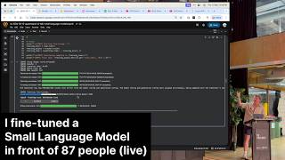
Small Language Models (SLMs) Are the Future: Fine-Tuning AI That Runs on Your iPhone

Introducing Sunny - A MedGemma-Powered Skin Health Tracking App (Kaggle Competition Entry)
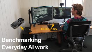
Benchmarking: NVIDIA DGX Spark & NVIDIA RTX 4090 | Part 4 - Comparing the results
Benchmarking: NVIDIA DGX Spark & NVIDIA RTX 4090 | Part 3 - Running LLMs on the RTX 4090
Benchmarking: NVIDIA DGX Spark & NVIDIA RTX 4090 | Part 2 - Formalizing the tests
Benchmarking: NVIDIA DGX Spark & NVIDIA RTX 4090 | Part 1 - Creating a series of tests
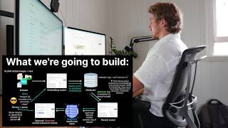

Local Multimodal RAG on the NVIDIA DGX Spark | Part 4 - Publishing our demo to Hugging Face


Local Multimodal RAG on the NVIDIA DGX Spark | Part 3 - Putting it all together