Comprehensive Logistic Regression Tutorial: From BASICS to ADVANCED
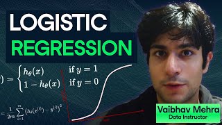
Viva Vera teaches logistic regression from sigmoid and cross-entropy loss through implementation on real datasets. The tutorial covers binary classification on breast cancer data and multiclass on the digits dataset, emphasizing the math before code.
Chapters
Hey guys, what's up? My name is Viva Vera and I'm an AI instructor here at datacamp. In this tutorial, we're going to be covering one of the most fundamental machine learning algorithms of all time, logistic regression. Now, in this one hour tutorial, we'll try to cover almost everything about it, such as the mathematics behind it, like maximum likelihood estimation, softmax, sigmoid, how to derive it from scratch, etc. But we're also going to be learning how to code it. So specifically using Sklearn. Now that pretty much will cover everything about logistic regression. So if you're ready to watch this and go on this journey with me, I will see you in the code. There's a lot to cover, but let's start off with the very, very basics. Now, there is one assumption I'm going to make. I'm going to assume you know a little bit of calculus already and what log functions are, et cetera. I assume most of you already know this, so this will be completely fine for you. You don't need to know any AI prior knowledge beforehand. Sounds good. Okay, let's start. So, logistic regression, it is one of the most fundamental machine learning algorithms for classification. Now let's actually dive into what classification means. Classification is about sorting things into different categories. Instead of predicting a continuous value, such as house prices, we want to predict what's called a label. Now some really, really famous examples are emails. For example, they could be classified into spam or not spam. Or for a patient, it could be healthy or they could be sick or an image. You probably have seen the dog or the cat classification example. Now each of these examples have two labels, such as dog, cat, healthy, six, spam, or not spam. Now there are many different types of classification. The simplest form is called binary classification, just like we just saw. All of these examples are binary classification because there's only two possible outcomes. But there is one step forward to it is called multi class classification. And here we have more than two categories or two labels, but each input only belongs to one. This point is really crucial. Each input only belonging to one class, category, label. They all mean the same thing, but the main point is they only belong to one of them. For example, predicting the color of an object, there could be many different colors such as red, blue, green, yellow, etc. But, but that object could only be of one color, assuming there's only one color on the object. Right. Then it could be classifying exam grades A, B, C, D, E, F, whatever, and image classification in Each image, if we're assuming there's only one object in each image, there could be an apple, a banana, an orange, a dog. You get the point. There's a third type of classification as well which is less understood and that's called multi label classification. Arguably this is the most important to industry. But. But we usually use logistic regression for binary classification and multi class classification. But coming back to multi label classification, because it's important for your knowledge, each input here can belong to multiple classes at once. So there could be more than two categories. There could only be two categories, but the point is each input can belong to multiple categories. So for example, for music genre classification, the music genre could be a mix of different categories such as jazz, blues plus rock. There could be an image where it has multiple different objects such as dog park, boar, and for a news article, it could be both about politics, economy, etc. Now hopefully you've understood classification, it's quite straightforward, but it was important to get it out of the way from the get go. But what if I say this now if I said logistic regression, most people would automatically think of linear regression and well, that is valid because they both have regression in their names, but they are actually quite different and this is a common mistake. So linear regression is used for predicting continuous values such as house prices, temperatures, salaries, etc. Whereas logistic regression is used for predicting categories or labels like spam or not spam, sick or healthy, etc. So one's predicting continuous values, the other's predicting categories or labels. This is very, very important. Now if we go into the mathematics, you hopefully you will start to see what the actual difference is. They are quite similar. But there is one small detail, well, not small, one detail which actually makes it into logistic regression. If we cover linear regression first and look at the linear regression formula, it really looks like a straight line. It's y equal to mx plus C or Y equal to mx plus B. Whatever you've learned. And this is obviously the simplest equation, there could be multiple different coefficients, right? But the point is it predicts numbers on a continuous scale, such as predicting exam scores from study hours. But if we look at the logistic regressions formula, take a look at this equation. It's very similar to the linear regression equation where you can see that this part is the exact same as this, but it's been wrapped by a particular function, this funny little thing, it's called sigmoid. Now this sigmoid function, what it does is it squeezes the output into between 0 and 1. Now, we're going to be covering sigmoid function in a lot more detail, have a lot of animations, but that's what it does. That's really the difference between linear regression equation and logistic regression equation. And a good example for this is instead of predicting the score to be 85, for example, it predicts things like 0.85 or 85% probability of passing. So that's what the sigmoid function does as an intuition. But now let's actually dive into the mathematics behind sigmoid function. So the mathematical function that allows us to turn any real number into a probability between 0 and 1. There are many types, but sigmoid function is quite famous. It's mathematically defined as this 1 over 1 e to the minus z. At first glance this might look confusing, but if we look at the graph, you can see it's actually quite simple. It's just a simple S curve. Obviously there's like different variants of it which we're about to cover. But there are two main things to this equation. One is Z, which is the input, and this could be the linear regression equation. But this only has two coefficients like the weights and the biases. But more generally, we write it as theta transpose X. Now obviously this is in matrix formulation. If you don't know matrix formulation, that is completely fine. But if you do, this should be quite familiar to you. And the second thing is Euler's number, which is equal to 2.718, et cetera. And that is also used here as a quick tip. Machine learning engineers and AI engineers like to use Euler's number and logarithms everywhere. So you should get very familiar with Euler's number and logarithm. Okay, so this is the sigmoid function shape. And you can see, like I just said, it's shaped as an S shaped curve. That's why it's called sigmoid. Now here are some very important details about this curve. For starters, for very negative values like these, it's very, very close to zero and it flattens but never actually touches it. There's an asymptote here at 0 at y equal to 0. For every positive number of x, it's quite similar, but the curve flattens near 1 where the asymptote again is y equal to 1. So it never really touches 0 or 1. It's always bounded in between it and right in the middle at x equal to 0, the function output 0.5. So it's perfectly balanced now the shape is also quite similar to other common activation functions such as Tanh function. Now, activation functions are used in neural networks or machine learning algorithms to try to add some non linearity into the function approximation. If you didn't know what that meant, that's fine. I'm just trying to show you basically what the sigmoid function is similar to other functions. For example, the Tanh function. And the Tanh function also has the exponentials and Euler's number within it. That's why it's a similar shape. Now the reason why the Tanh function looks quite similar to the sigmoid function is because they both contain Euler's number. I didn't include Tanh's function mathematical formulation here because I didn't want you to get confused and you don't really need to know it. But just remember that as some new knowledge. Now let's talk about some key properties of the sigmoid function. So this is the sigmoid function. Again, these three details are quite important because this is why we use the sigmoid function here. Number one, it's smooth and differentiable. It's perfect for gradient based learning because, well, one of the most common optimization algorithms in any machine learning algorithm is gradient descent. And gradient descent heavily relies on continuity and this is perfect for gradient based learning. Number two is its squashes the value between 0 and 1. And the reason this is important is because no matter how big or small the input is, it always stays within this range and this allows for more stability in learning. And number three is thresholding effect. Small negative inputs become almost zero and large positive inputs become almost one. So it penalizes large errors quite heavily, which is a good sign. Now obviously the shape can differ based on the coefficients you write. So for example, if we go back up to the formula, if Z, or more formally, these theta values are different values, they'll obviously change the shape. And that's what we're about to look at now. So now I'm going to show you two animations. The first will be to build your intuition on how a line gets converted into a sigmoid function in the first place. If we go here and play this animation, you can see that that was a line and it got converted into a sigmoid curve because we wrapped it around the sigmoid function. Now, if we have a different line like this, you can see that the shape, the S shape, is still preserved. Obviously it's reflected now because the gradient was negative in this case. But you can see that the Shape you can still see. And if we use another line, for example, this time a lower gradient line, you can see that the S shape is almost flat. And that brings an important point here. Only when the line depends on X example Y equal to X, Y2X, et cetera, does the sigmoid transform it in to a S shaped curve. So what does that mean? Well, it means this. If Y was just equal to a constant like Y equal to zero, it will basically, well it won't change because there is no gradient. So the point is there needs to be gradient or non zero coefficients of theta values for it to actually have a little curve or an S shaped curve. So that is an important point to remember. Now I want to go back to linear and logistic regression one last time and that is to build your visual understanding. So the Y value values are the probabilities of X being in class one. Speaking of binary classification for now. So I want to show you why linear regression doesn't really work for classification tasks. And that is with this example you can see that I have a data set with two classes, yellow and blue. So the yellow class has label one and the blue class has label zero. Now if I draw a linear regression using a linear regression algorithm, the best line or the line of best fit is this line. We're predicting values or probabilities over 1 and less than 0, which doesn't make any sense because that defies what probability actually means. But take a look at how the line changes when we add a sigmoid function. So if we continue playing, you can see that the same line now is converted into an S shaped curve. And that is what logistic regression is. From a visual perspective you can see how the probability shifts that is goes towards 1 as the class label as more and more density, as there's more density of Class 1 labels around this region of around X being positive. Now obviously this was quite a simple example because this was binary classification. But it's important to have a start building your visual understanding right from the get go. So hopefully this animation helped you. I want to keep building your intuition here by doing a simple example with you. So let's mathematically solidify this now by looking at this. Suppose we have a straight line which is Y equal to one, which means every input X maps to the constant value 1. If we pass this through the sigmoid function which was this, all I've changed is the variable name, right? So now it's Y. But before it was Z. And if I input 1 now by y equal to 1, you can see we get 0.731. So since every X gives the exact same Y equal to one after sigmoid, every X will give the same, well, same value, meaning we again get a horizontal line. And this is what I was saying on this point, that we need some X coefficients, not just a point single constant like y equal to 1, y equal to 0, etc. So hope now that mathematically proves why we also get a horizontal line. So in case if you were wondering, this is the reason. Now hopefully you're at a point where you actually can visually understand or have a little bit of an intuition as to why we use logistic regression over linear regression and what the sigmoid function actually does. You can play around with the values. I highly recommend this playing around the values and seeing how the shape changes and trying to prove this yourself as well why this is true. So once you've done that, we're now going to be covering the cost function. Now in this section we're going to start off by asking you a question. Why not MSE or mean square error? After all, mean square error is one of the most common and famous cost functions in all of machine learning. Why wouldn't it be a good fit here? Especially because MSE or mean square error is the cost function for linear regression. Well, let's test this idea together. Below is this mean square error formula. You can see that means here one over M. The two is here for when we differentiate this, these two will cut out. It's just for making it easy. And you can see that this is our predicted value and this is the actual label we square it. It's pretty self explanatory right now this works great for linear regression because of this fact. The error surface is convex, AKA a nice bowl shape. But in logistic regression, H theta X is sigmoid theta transpose X. But now that we've added sigmoid, making it a non linear curve, the error surface is non convex. A non convex 3D surface is something like this, which the main point I'm trying to make is there are lots of local minimas. There's no one global minima like in a convex or nice ball shape. So this is a visual reason why we can't really use mse because we're most likely going to end up in a local error. And that is obviously quite problematic. And that is what I've said here, that non convex is problematic because there are lots of local minima, which means our optimization algorithm, which is gradient descent can get stuck. And this means that the training becomes unreliable. So what can we do to solve this problem? This is where maximum likelihood estimation comes in. Now I've written an article already on tataCamp. If you want to check it out and you prefer text way, you can check it out here. But I'm also going to briefly cover it here as well. So, to derive the loss function we need to use maximum likelihood estimation and we're going to assume that Y follows a Bernoulli distribution. Now, Bernoulli distribution sounds complicated, but it's really the most simple probability distribution out there. It basically saying with this complex looking maths is that our label can either be 1 or 0. That's all it means. Okay, again this conditional probability, it looks scary, but all it's saying is with the given values of x, AKA our features, what is the probability that y belongs to class 1 or Y belongs to 0? Now, H theta X, remember is this sigmoid transp. Sigmoid theta transpose X. So again, if you need to rewatch this, go ahead because this is important. Bernoulli distribution is the foundational block of how we derive the cost function going on for binary classification. For binary classification specifically, for example, if the probability of getting 1 was 0.7, aka h theta x, or this gave us 0.7, well then the probability of getting 0 would be 1 minus 0.7, aka 0.3. Why 1 minus? Well, two reasons. One, again, if we look at the piecewise function, it says that 1 minus 0.7 is 0.3. And from a more intuition perspective, again, 0.7 and 0.3 have to add up to 1 because there's only two possible outcomes, right? 0 and 1, and it has to be a valid probability distribution. I know, I'm trying to go over this again and again, but this is important. If you understand this part, everything else should be easy. Now let's move to step two, which is the likelihood of a data set. Now people often get confused between likelihood and probability, and it is a confusing concept. But I'm going to try to cover what the difference is here. The likelihood measures how probable our data is given the model parameters theta. So in plain simple words, if these weights theta were the true parameters, how likely is it that we would see the labels in our data set? Again, if y1, this simplifies to H theta X. But you could be asking, well, what does this power? I mean, it just means what observation or sample we're on. So I is just an index. So it could be the first first observation, second observation, etc. We have lots of samples, right? So if we have, let's say 100 samples in our data set, I could be the first sample, the second sample, all the way up to 100 sample. And again, if y was equal to 0, this simplifies to this. Now here comes the most important part. Bernoulli distribution was important, but this arguably is more important. We assume that all samples, or m samples, like 100 samples, 10 samples, however many samples there are in our data set, are independent. Why? Because when we can just multiply these probabilities together, why can we just multiply these probabilities together? Well, this is what's important. Most people miss this point. What you're actually doing is conditional probability. And there's a reason for this. Your Y label in this case, 1 or 0 is dependent on what the features were, right? The X features, like for example, if I was doing a pass or fail, like 1 or 0, there could be lots of different features such as how much the student's IQ is, what was the student's height or whatever Height probably doesn't have a correlation, right? But like you can see, there are different features which contribute to what Y could be either 0 or 1. And that's what we try to approximate. That is why this is a conditional probability distribution. This looks more complicated than it is, but it really is simple if we look at it in a more intuitive way. Again, Y is condition on X on the X features and it's parameterized by theta. That is all this is saying. And hopefully that grade or pass or fail example which I said helped you build your intuition here. Now, because we made the assumption that all of these M samples are independent, this is basically saying that, for example, sample one is, and sample two, they're not dependent on each other at all. Like they're completely independent, right? So that means we can just multiply their probabilities together. Otherwise it would mean something like this if we have two samples in our data set. So Y, let's say Y is equal to 1 for the second sample would be condition on X on the features of the first sample and the features of the second sample and this. So that would be a comma here. And that would make it so complicated. Think about M being quite a large value. There would be so many different conditions we would have to do conditional probability on. But because that is not a thing, we can just simply multiply them with each probability Y being only honest respective samples feature. So hopefully that makes sense to you. And this entire product is Called a likelihood function, it tells us how good of a choice theta is at explaining the whole data set for logistic regression. Since each label yi is assumed to follow a Bernoulli distribution, the probability of one sample can be written like this. We don't write it in a piecewise function, we want to make it a more continuous function. So this is a continuous function, right? And this is a very, very, very clever way of writing the same piecewise function. And I like to think of this analogy as a light switch. We're going to do an example together, but I just wanna again build your intuition here. All right? So this is quite awesome. So if we look at this more in depth, I like to think of this as a light switch analogy. Now we're going to focus, we're going to do an example together in just a bit. But I just want to build your intuition first. So in this light switch function, I like to call it that, but it's not actually like properly defined as that. But I like to call it that Y can either be 0 or 1. Let's say if y was 0, the important thing to note here is that H theta x is for label 1 and 1 minus h theta is for label 0, right? So if y was equal to 0, which one of these would we want to like activate? We would want this value to be multiplied to the all of the samples probabilities, right? Because this is what tells us the probability of that being 0 of that sample being 0 or in label 0, right? Similarly, this we want to be activated, I say activated in quotations. But this is what we want to be multiplied with the different with all the other samples. Because this is the probability of that sample being in label 1. 1 minus H Theta X is the probability of that sample being label zero. And we want to activate this when we Y to be zero, right? And H theta X, we want to activate that when we know that this label is one. So this is why this is clever, because if we substitute Y equal to zero here and we do whatever what, and we do this value to the power zero, anything to the power of zero is just one, not zero. It's to the power it's equal to one. And because of that, if we do this one minus zero, one minus zero is just one. So this just stays preserved. So what we're doing is 1 times 1 minus H theta, which is actually the probability of that being in label 0 with probability of being labeled 0. Similarly, if y was equal to 1 and we do this, we want this to be Activated. So H theta X to the power of one is just itself. But here, because one minus one is zero, this becomes one. So that is quite clever. And if you still don't understand, hopefully this mathematical example will make sense. Now this is a very simple data set, but, but let's assume that within our three samples, two of those samples are in class one and one of those samples are in class zero. And this is their respective probabilities. Now, H theta X is what our model has predicted for it to be in class one. Because remember, H theta X is the probability of that feature or that sample being in class one and that it's given as 0.8, 0.7 and 0.4. So it's quite wrong for this one for the second and the third sample. Right? And if we want to find the actual probability, this would be the same, and this would be the same and this would be 1 minus 0.7, because this is in label 0 and there's only two outcomes. So 1 minus 0.7 is 0.3. Now if we use this formula, you can see that we get 0.8 to the power of 1. Because look at this. H theta x for the first sample is 0.8 to the power of what the label is. The true label is 1 multiplied, which is this term 0.2, because 1 minus h theta x is 0.8. So that becomes 0.2 to the power of 1 minus 1, which is 0, and that becomes 1. And we can do the same thing for second sample and third sample. And when we do that, you can see we can just simply multiply their probabilities together. So 0.8 times 0.3 times 0.4 is equal to 0.096. And this is clever. I want you to use the same data set and try to get the same answer again. Or you could even create your own data set and try to come up with the answer yourself as well. But this is important and hopefully you can see why I called it the light switch function. And hopefully you can see why I called it the light switch function unofficially, because due to its binary nature, it switches on which term, it switches on which term depending on what the sample's true label is, 0 or 1. Now this only works for binary classification, obviously we're going to see how it works for multi class classification in just a bit. But this should hopefully make sense to you now. But like all things, there are some problems and this is what we're going to be covering now. So number one, the likelihood is a product of many small probabilities. Each of these are quite small values. 0.8, 0.3, 0.4. They're just probabilities, right? But it quickly becomes a tiny number. And the reason is if we multiply lots of these terms, it is harder to work with because it keeps on becoming smaller and small. In just three samples we reach 0.096. If we had 100 samples, which still is quite a really small data set, just think about how small this value would be. The reason this is really bad is because when we take the derivatives, which is needed for gradient descent, the change would be so small that we basically learn nothing. And that is the reason why we don't use multiplication here. So we need to try to find a way to not use multiplication but still get the same sort of thing. That is where the log function comes in. Logs make maths a lot easier. It also makes the gradients not become as small because it makes the multiplication into addition. And that is hugely beneficial. So the formula becomes this. Now why does the formula become this? Well, this is still straightforward maths. The product becomes summation. The powers were this y and one Y is just a simple log identity which brings it down. And so that's why we get it like this. Now let's do a quick mathematical example to get familiar with this function. So again, the same data set here. If we now use this formula, and this time I've also put the average here, this will become the log loss function. So you can see when sampley is equal to 1, the probability 0.8, we do log of 0.8. We get this similarly with 0.3, not 0.7 because this is in plus 0 and this will also be 0.4 and we'll get these values and when we add all of these values we get something like this. Please also note that I've also included a negative sign here. You will see why in just a bit. But the main thing which I want you to note is look how better this 0.781 value is than the very small 0.096 value. And the reason this larger value is more beneficial is because when we do backpropagation, that means we'll be able to learn more quickly. Hopefully that all made sense. The final step is cost function. And that is what I just wrote here, minus 1 over M. And the reason we use negative is because we're performing gradient descent. So we don't want to find the maximum, we want to find the minimum value. If we didn't do minus we would need to do gradient ascent and that would be slightly confusing. You can still do it, it will still work. But to follow the convent we use the negative and we've performed gradient descent and that's why we multiply negative one. So this was the final form of the logistic regression cost function and it's also known as the cross entropy loss. So that was a lot of maths and I really want you to rewatch it and try to derive this yourself using a pen and paper. Once you've done that, try to come up with your own data set and try to work out all the values. You will learn a lot faster. Once you're done with that, we can go into the coding. Now, there is one important point which I want to raise here, which is when we start the coding, you will see that a lot of the underlying code which we are supposed to do ourselves is already covered using Sklearn. And in industry we do use Sklearn and all these libraries because it makes our lives much more efficient. So the point which I'm trying to make here is a lot of people think we can just skip the maths and go straight into coding. And that is a bad approach because trying to learn machine learning algorithms without knowing maths is, well, you're not going to get anywhere because you're not going to understand the underlying architecture. If you want to be a machine learning researcher or engineer, you really need to know the mathematics. Coding is important, but without the mathematics, well, you really can't get anywhere within and you won't be able to contribute to research if you don't understand the fundamentals like logistic regression and etc. So the point I'm trying to make is you should understand the mathematics and focus on that much more than trying to implement and code it yourself. Mathematics is going to get you far. Not coding, because coding we can just use ChatGPT nowadays. Right, so that was the motivational speech. Okay, to code this. Now we're going to use again scikit Learn and you need to pip and solve these libraries. I'm using per Python version 3.12.6, but these libraries are quite stable and you should be able to install it quite easily. Okay, let's begin. So we start off with all of these different imports and we're going to be using this breast cancer data set for this because it could either be benign or malignant, either zero or one binary classification. Once again. So first we're going to load the data set and you can see that I've printed the Data here. And now we're going to put it into X and Y. X and Y is a really common convention when we're doing machine learning algorithms. So X are the features and Y is the actual labels. So if I print X and Y instead of data, you can see that this is the X value and this is the Y value, the X value. There's a lot of different features, right? And similarly for Y, there is one label per sample and these are the number of samples we have. Now, if we progress further, we first scale these. And the reason we scale these is it makes training much more stable. And to implement this again, we can just use the sklearns inbuilt functionality inbuilt method, which is fit transform and we convert X. Now, this is a very common mistake. Don't scale the Y values because that doesn't make sense. It should either be 0 or 1 for a binary classification. Right? Like whole numbers. If we use the scaling. If we use scaling, it will completely mess it up and ruin everything. Right? So don't do that, just scale X values. And now we split it into train test. And I want to briefly mention this here. You've probably heard of training and testing datasets. You might have heard of validation dataset as well. I'm not going to be including validation dataset here because that's not the main point of this. The main point is to learn logistic regression. Right? But I'm still going to cover these parts. So just before I cover this, there are a few parameters which I want you to see. The first is obviously X, Y and test size. Now, test size, random state and stratify is what we're going to be covering right now, starting off with test size. So imagine this is our data set. Test size says what proportion we want to send into our testing data set to see if we've overfitted or underfitted, or if we haven't overfitted or underfitted to make sure. And in this case, because we've got the test size to be 0.2, it means 20% of the data will be used for testing and 80% will be used for training. This is a very common ratio which is used in when we're doing machine learning. And again, we've left validation for now, random state equal to 1. This makes results reproducible. If you set the same random state as I have, you will get the exact same results as I do. The values will be the exact same. So it's really just for reproducibility. You don't need to include this parameter. It's not like a fixed, it's not a parameter you need to pass in. But if you want the same results as me, just put random state to be one. And lastly, stratify. And we've put stratify equal to Y here. So this basically makes sure that the class ratio, either benign or malignant or 0 or 1, is balanced in both training and testing data sets. Balancing data sets is something which people often miss and it could be one of the reasons why your algorithm is not performing well. A good, well balanced data set is important. Take a look at this example. Imagine we have a mini data set which has 100 samples. So it has 80 benign and 20 malignant samples. And we have a test size of 0.2. Now this means we're going to be having 80 training samples and 20 testing samples because again, 20% of our data we'll be going into the testing data set. Now, without stratification, you can see that in training there will be 70 benign samples and 10 malignant samples. But in the testing there will be 10 benign and 10 malignant. And this is unbalanced. Obviously you might think that, okay, that's fine, but this is a quite a small data set. Think about data sets which are billions and billions of samples, right? With stratify you have a more balanced. And what I mean by balanced, I mean proportions are balanced. So the proportion of benign to malignant is the same in the training and testing dataset. It keeps the 80:20 ratio. So TLDR is this. Stratify keeps the class balance the same in training and testing datasets. And this allows the model to learn and evaluate fairly. So that's why we use Stratify. Cool. Now if we progress further, this just this one command will be able to perform logistic regression for you using Sklen. And this max iteration parameter is. I've set it to 500. I think the default is 100. That doesn't really matter. But the point is higher iterations are used for convergence. But. But the key limiting factor is that it could be overfitting. So you might get really high results on the training data set, but on the testing data set you might fail because you've iterated so many times that it's overfitted. So now we fit this and we fit the model on the training data first. So xtrain and Y train. Right? So let me quickly run all of these and you can see that we've got this. Now let's go on to predict Stuff. So y prediction is equal to model predict X test these simple commands in just few commands. We've been able to train our own logistic regression model using Sklearn. Right? But again, maths is the important point. If we print out the accuracy scores now, you can see that we got on our Test data set 90.0.9912, which means 99.1% Accur. Now, breast cancer data set is quite a small data set, but that is still pretty impressive, right? I guarantee you that if you didn't do stratify or you didn't do standard scale at the scaling thing, you might get a slightly worse result. Not by a lot because this again is a small data set. But stratify and scaling are two important techniques we can use to make our results better. And using classification report, which is another inbuilt method in Sklearn, we can print out the confusion matrix. Now this confusion matrix looks a bit ugly, so I used Seaborn to be able to make it look pretty. It's just for aesthetic reasons. I just like Seaborn because it looks nice, but it's saying the exact same thing as here. You can see that out of the in for this is only for testing. So in our testing sample we had 41 where we predicted malignant completely correctly. We predicted 72 benign cases completely correctly. But there was one where we predicted benign but it was actually malignant. And that is really, really bad. So we don't want this, right? We would much rather have it we predict malignant but it's actually benign than the other way around. Well, obviously best case scenario is we predict everything correctly, but that is often very, very hard to do and just almost impossible. But that was what the confusion matrix is. Obviously we can go further in depth and talk about precision, recall, F1 score, etc. But there's no point in that. The main focus was logistic regression and that is how you code logistic regression for binary classification purposes using Sklearn. But at the start of this tutorial I did promise that I will be going into multi class classification using logistic regression, which is less frequently used. But the mathematics is, well, it's fun. So we're going to be covering that as well. So I'll see you in that section. So let's quickly recap what we just learned about the binary logistic regression. Again for two classes, 0 or 1, the model assumes this. Again, we talked about this in quite a lot of detail that given for example y equal to 1, its condition on x parameterized by Theta, it's equal to this sigmoid function and again its complement, or for Y0's case, it's equal to this. So there's only one weight vector here, theta and sigmoid guarantees that the probabilities add up to one. Now for multi class classification though, don't use the sigmoid function, we use the softmax function. And I want to take a brief pause here and try to look at the softmax function in a bit more detail. Now the softmax function is quite possibly one of the, if not the most popular function in AI. It's so, so commonly used mainly because of its one property. It can convert anything into a valid probability distribution. Obviously not everything like apples or bananas, but you can try to see like what I mean here. It basically turns your raw scores, or more technically speaking, logits into a valid probability distribution. Now let me ask you a question. What exactly is a valid probability distribution? Well, the values. There's two things. One, each value has to be between zero and one. And number two, when you sum up all of those probabilities, they have to equal to 1. And softmax function does that perfectly. So again, it's a multi class version of sigmoid. It turns the raw scores or logits into probabilities that are positive and add up to one. Let's do an example together. Predicting exam grades. So let's say our model, the raw outputs or the logits for a student belonging to one of three grade categories. Is this so? What that means in a more layman term is let's say I pass in some features about that student and I've got a model and I predict it these values for that student getting either grade A, B or C, and these are the raw scores. Again, this is not a valid probability distribution because, well, it's positive, but it doesn't add up to 1. So we compute the exponentials because using this formula we do E to the power 2.1, e to the power 1.3, e to the power 0.2. You get the idea. And then we normalize. Now why normalize? Because if we scroll up up and look at the formula once again, you can see this term, the denominator term where we have to sum up all of these exponentials. It's basically just making it into ratios here. What proportion of all of the logits was grade A? We'd use exponential here and not just sum them up because what if these were negative? That would have made the denominator less than the numerator, right? Because if we had like minus 0.2, the denominator would be slightly less than if we did plus 0.2, for example. So that wouldn't correctly identify the proportion of the magnitudes of these grades or logits. And that's why we use exponential. And you can see after doing all of these normalizations, we get these as the final probabilities. So this is a 63% probability that that student ends up in grade A. And obviously probabilities are much more intuitive because outputting a raw score of 2.1 and 1.3 and 0.2 like it doesn't really make sense. But if I say oh, that student has a 9% chance of getting a grade C based on the features, which I, it makes much more sense and is much more useful. So the model predicts that the student is most likely to get grade A because, well, it's the most probable value. And notice how this is a valid probability distribution. Now, now that we've covered softmax function in quite a lot of detail, let's progress onwards. There's this one important point which I want to make, which is that imagine we have K classes. So 1, 2, 3, all the way up to K could be like 10, 100, whatever. Each score for class K would be given as this and the softmax probabilities would be this. Right? So let's say probability of Y being in class three, given all those features and parameters parameterized by theta would be the softmax function. In binary classification it was sigmoid. Hence if it was k equal to 2, it would reduce to sigmoid. Now a homework question for you is try to mathematically prove that Y when k is equal to 2, this is converted into a sigmoid function. It's quite fun, little bit challenging, but it will help build your understanding much better. So that's your homework task and tell me if you've done it in the comments below. So once you've done that, we're now going to move into the likelihood functions. Now please, this does look very terrifying, but if we just look at it for slightly longer, you will try, you will see how it's quite similar to what we just covered. Good. So for binary this was exactly what it was earlier, it was hdx. But this is the exact same, right, because this means class label 1's probability and this means the sample being in class 0's probability. But in multiclass this is. We can't do this because this light switch analogy, well it was either on or off 0 or 1, but because now we have more than two classes, K classes. We use something called an indicator function. Now if this is the first time you've actually heard of indicator function before, think of it as an if else statement. So if the condition inside the bracket is true, then the output is one, but if it's false, then it's zero. Okay? That's all it is, a simple if else statement. So let's take a look at this multi class in a little bit more detail. Okay? But another difference is this. Notice how we went from being either 0 or 1 to this. This is basically the same thing. It's literally just conditional probability. Again with the conditional probability being y equal to belonging into, let's say class three with these parameters and this. Now if you fully understood the intuition behind this, this should also be quite easy to understand. What we're really doing is once the probability of that class has been obtained, let's say we found the probability of Y being in Class 3, right? Only that probability is used. All of the rest is just one for that sample. So that's why we have this product. So if we had three categories, 1, 2 and 3, and let's say the true class of that sample was, let's say k equal to 2, then for the first class for that sample it would just be 1, because this indicator function would give us 0 and anything to the power of 0 is 1, so it'd be 1 multiplied by the actual product probability which we've got because it's the correct class, because these classes match. So that will be this probability multiplied by one. Again, because this is the third class and the third class is not the correct class classification here for this sample. So if we do one multiplied by this, multiplied by one, well we just get this for that sample and if we now go into the outer loop or outer product, you will see that we have to do this for all m samples. So again then all we're doing is finding the correct probability of finding the probability which are model predicted. So all we're doing is finding the probability for that correct class for every single sample. So again we're finding the probability for every single class for every single sample. That's all we're doing. Okay, but like we covered last time, these values will become so small, especially if n is quite large. And that is why we have to use log likelihood once again. We convert this into a log function. So like in binary log likelihood, it's the same with multi class log likelihood. And you will see that the indicator function where it was in the Power it's now been brought down because of log identities and we get this and we can just simplify this to equal to -1 over M. Again we put the negative because we want to minimize this function, not maximize and then we can just perform gradient descent. Now I'm not going to cover gradient descent here because that. Well, the main part which I wanted to cover was this part gradient descent. You should already know we will just use back propagation to be able to update these weights or theta weights. And so that is the cross entropy loss or the cost function for multi class logistic regression. In summary, I want you to remember these three points. Binary is sigmoid and multiclass is softmax. And the cost function generalizes from binary cross entropy to multiclass cross entropy. Now if you want to slightly understand cross entropy more, I've also written this article on KL divergence where I go deeply into what entropy and cross entropy are in again as an article. So do check that out if you want to understand more about cross entropy. But let's progress onwards now. Okay, so let's code this up and the code is very, very similar. Again we're using Sklearn and if we're quickly run this. So the imports as you can see are quite similar as what we did before. Obviously the data set will be completely different because well the breast cancer one only had two classes but this lowest digits class has 10, aka 0 to 9. So it's basically trying to predict what class the features will be 0, 1, 2, 3, 4, 5, 6, 7, 8, 9. Okay, and that is what we do here. We load the digits and place it in X and Y. Now we split it into train test and we do X Y test size equal to 0.2 and random state equal to 42. Now yes, I deliberately left out the stratify and the scaling and that will be your homework task. So all of this code will be in a GitHub repository and you can find that GitHub repository in the description below. So do that homework task, it will help build your intuition further. Now again we just train this multinomial logistic regression with max iterations as 2000 and these two parameters. This is a solver which Sklearns use to optimize stuff you don't need to know about it and we just fit this model and once we've done that we can predict stuff and you can see that we get a classification report here. And this is basically saying The Precision Recall, F1 Score and Support of all of these digits. Now Again, I'm not going to be covering the Precision Recall F1 score of the support values here because it's really just not needed. But I will show you the confusion matrix. So you can see the confusion matrix is a lot bigger because well there's 10 classes and 10 by 10 matrix now, right? And you can see that we've performed quite well. There are obviously the odd ones here on both sides, but you can see for the vast majority we've predicted it, right? The reason I can tell that because 9, the predicted 9 corresponds to the actual 9 value, right? So that's why it's all in the diagonal. And so this is just a visual way of seeing how well our models perform. And from the looks of it, it performed quite well. Another homework for you is to actually give me the actual accuracy of this. And that's all well done for finishing this tutorial in such a short amount of time around one hour. We've covered so much. So we covered the key terminologies such as Softmax and Sigmoid. We found the difference between logistic regression and linear regression through those animations and mathematical formulas. We derived the loss function of logistic regression using MLE maximum likelihood estimation. We introduced that that we coded logistic regression using Sklearn and we also coded multiclass classification and we looked at its formula as well. So well done again for doing this. But please remember that mathematics is important so try to derive all of the binary classification and multi class classification yourself as well. It will help you in the long term. Now, where to go next? I highly recommend these two courses, the supervised machine learning course because well, logistic regression is a supervised learning is in supervised learning. So I would highly recommend to understand all of supervised learning machine learning algorithms. I would highly recommend this course on datacamp and I would also highly recommend if you want to gain more conceptual knowledge about machine learning as a whole, I would recommend this course. And again if you want to more text or more article based approach, then you can check out the two articles which I mentioned previously in this tutorial. And that is all. Now if you have any criticism or any feedback about how this class was taught, put in the comments below, check out the description for the code and I will see you in another tutorial. Bye for now. Sam.
More from Richie

#359 My Best Friend is AI with Valerie Tiberius, Professor of Philosophy at University of Minnesota







How AI Agents Will Work While You Sleep | Ruslan Salakhutdinov, Professor at Carnegie Mellon

#358 How AI Agents Will Work While You Sleep | Ruslan Salakhutdinov, Professor at Carnegie Mellon

