In this introductory lecture, Dan Becker—a data scientist and contributor to Keras and TensorFlow—explains why deep learning, particularly neural networks, are superior to simple linear regression for predictive modeling in a banking context. Using the example of forecasting the number of transactions a customer will make next year, he shows how linear regression assumes additive, non‑interactive effects of features such as age, balance, and retirement status, resulting in parallel prediction lines and unrealistic assumptions. He contrasts this with neural networks, which model complex interactions through hidden layers, allowing non‑parallel, more realistic predictions. Becker outlines the course structure: the first two chapters cover conceptual foundations (including how hidden layers aggregate information and why more nodes capture more interactions), preparing students to debug and tune models; the later chapters focus on practical Keras code that replicates and extends traditional Scikit‑Learn workflows. The lecture emphasizes that deep learning’s ability to capture intricate feature interactions underpins its success across text, image, audio, and code domains, setting the stage for hands‑on model building later in the course.
Chapters
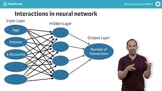
I'm Dan Becker, a data scientist and contributor to the Keras and TensorFlow deep learning libraries. Imagine you work for a bank and you need to build a model predicting how many transactions each customer will make next year. You have predictive data or features like each customer's age, bank balance, whether they retired, and so on. We'll get to deep learning in a moment, but for comparison, consider how a simple linear regression model works for this problem. The linear regression embeds an assumption that the outcome, in this case how many transactions a user makes is the sum of individual parts. It starts by saying what is the average? Then it adds the effect of age, then the effect of bank balance, and so on. So the linear regression model isn't identifying the interactions between these parts and how they affect banking activity. Say we plot predictions from this model. We draw one line with the predictions for the retired people and another with the predictions for those still working. We put current bank balance on the horizontal axis and the vertical axis is the predicted number of transactions. The left graph shows predictions from a model with no interactions. In that model, we simply add up the effect of the retirement status and current bank balance. The lack of interactions is reflected by both lines being parallel. That's probably unrealistic, but it's an assumption of the linear regression model. The graph on the right shows the predictions from a model that allows interactions and the lines don't need to be parallel. Neural networks are a powerful modeling approach that accounts for interactions like this especially well. Deep Learning the focus of this course is the use of especially powerful neural networks. Because deep learning models account for these types of interactions so well. They perform great on most prediction problems you've seen before, but their ability to capture extremely complex interactions allows them to do amazing things with text, images, videos, audio source code, and almost anything else you could imagine doing data science with. The first two chapters of this course focus on conceptual knowledge about deep learning. This part will be hard, but it will prepare you to debug and tune deep learning models on conventional prediction problems, and it will lay the foundation for progressing towards those new and exciting applications. You'll see this payoff in the third and fourth chapter. You'll write code that looks like this to build and tune deep learning models using Keras to solve many of the same modeling problems you might have previously solved with SciKit. Learn. As a start to how deep learning models capture interactions and achieve these amazing results, we'll modify the diagram you saw a moment ago. Here there is an interaction between retirement status and bank balance. Instead of them separately, affecting the income. We calculate a function of these variables that accounts for their interaction and use that to predict the outcome. Even this graphic oversimplifies reality, where most things interact with each other in some way. And real neural network models account for far more interactions. So the diagram for a simple neural network looks like this. On the far left, we have something called an input layer. This represents our predictive features like age or income. On the far right, we have the output layer, the predictions from our model. In this case, the the predicted number of transactions. All layers that are not the input or output layers are called hidden layers. They're called hidden layers because while the inputs and outputs correspond to visible things that happened in the world and that can be stored as data, the values in the hidden layer aren't something we have data about or anything we observe directly from the world. Nevertheless, each dot called a node is in the hidden layer represents an aggregation of information from our input data. And each node adds to the model's abilities to capture interactions. So the more nodes we have, the more interactions we capture.