Learn how continuous random variables work using Albert Michelson's 1879 speed-of-light measurements. The normal distribution shows a 3% probability of measurements exceeding 300,000 km/s, while the cumulative distribution function reveals a 97% chance of staying below that threshold.
Chapters
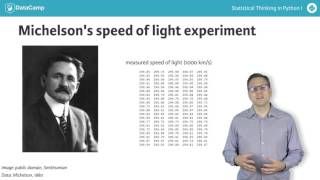
So far we have talked about probabilities of discrete quantities such as die rolls and number of bus arrivals. But what about continuous quantities? A continuous quantity can take on any value, not just discrete ones. For example, the speed of a train can be 45.76 kilometers per hour. Continuous variables also have probability distributions. Lets consider an example. In 1879, Albert Michelson performed 100 measurements of the speed of light in air. Each measurement had associated some error with it. Conditions such as temperature, humidity, alignment of his optics, etc. Change from experiment to experiment. As a result, any fractional value of the measured speed of light is possible. So it is apt to describe the results with a continuous probability distribution. In looking at Michelson's numbers shown here in units of megameters per second or thousands of kilometers per second, we see that this is indeed the case. What probability distribution describes these data? I posit that these data follow the famous normal distribution. To understand what the normal distribution is, let's consider its probability density function or PDF. This is the continuous analog to the probability mass function, the pmf. It describes the chances of observing a value of a continuous variable. The probability of observing a single value of the speed of light does not make sense because there is an infinity of numbers, say between 299.6 and 300.0 megameters per second. Instead, areas under the PDF give probabilities. So the probability of measuring at the speed of light is greater than 300,000 kilometers per second. Is an area under the normal curve parameterizing the PDF? Based on Michelson's experiments, this is about a 3% chance since the pink region is about 3% of the total area under the PDF. To do this calculation we were really just looking at the cumulative distribution function or CDF of the normal distribution. Here is the CDF of the normal distribution. Remember that the CDF gives the probability the measured speed of light will be less than the value on the x axis. So reading off the value at 300,000 kilometers per second, we see that there is a 97% chance that a speed of light measurement is less than that. So there is about a 3% chance that it is greater. We will study the normal distribution in more depth in coming exercises. But for now let's lets review some of the concepts we've learned about continuous distribution functions.