Webinar: Intro to Python for Spreadsheet Users
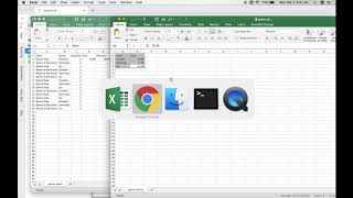
Chris Cardillo shows spreadsheet users how to move their work to Python using JupyterLab and pandas. He reads CSV files, joins them like a VLOOKUP, creates a revenue column, and builds a chart. Then he converts the notebook to a script that runs from the command line, automating what would take manual steps in a spreadsheet.
Chapters
Hi, how's it going? My name is Chris. I'm a data scientist here at datacamp and author of the course Python for Spreadsheet Users. I'm here today to walk you through a jupyter notebook that goes over some of the concepts that we teach in the course and looking forward to sharing it with you. So with that, let's hop right in. I have Excel open here just so I can reference some documents that we'll be using. But essentially, I think a good place to start is that while you're used to an app like Google Sheets or Microsoft Excel to do your spreadsheet work, I think a great place to start iterating in Python for the same end goals is a jupyter notebook. So there is no icon down here for a jupyter notebook, there is no app icon. So what you actually have to do is jump into your terminal. So this is probably the more intimidating part if you're just getting started. But if you get through literally three or four command line prompts, you'll be well on your way. So here's my terminal. This little tilde means that we're in my home directory. So if I was to look here, Chris Cardillo. So that's Chris Cardillo. And here's all of the folders that are available to us and files that are available to us. And if we do the command ls, it'll list everything that's in this folder. So I want to get to my desktop, right? I want to get here because all of the stuff we're going to work with is in this folder called Live. So to change the directory, we use the command CD and then a space and then the command line is case sensitive, so capital D des. And then I'm going to tab to complete, and if I hit enter and I hit LS again, you'll see now we've got this live folder here and then my actual desktop folder. So that's where I'm keeping everything. You know, I have a dirty desktop and I just swept it all under the rug. So that's what's in there. And so now if we wanted to get into the live folder, which is ultimately where we want to be, because it's where our files are and it's where our notebook is. We're going to use CD one more time and we'll do CD Live. And if we do ls, you can see, hey, we're in this live folder with game prices, game sales and live notebook. And so very quickly, what I'm going to do is let's do it again, but let's do it in one step. So you can actually do CD desktop and then you'll see the backslash there. And then we do backslash live. And then now we just went from our home directory into live and so now you can see that we're there as well. I'm also using Control L just to clear the command prompt. And so now we're in the right folder and it's time to launch our jupyter notebook. I like to use Jupyter Lab, which is essentially allows you to use jupyter notebooks, but also gives you like a file browser or the ability to launch console a terminal from in here as well, or a text file. So there's a lot of Handy features with JupyterLab, but we can now just. And again, just to draw the parallel, here is our notebook and here's our notebook and double click it and here we are. So this is the notebook that I prepared for this session. So let's go through what's here. So first and foremost, what is Python? I think in three parts we can describe it as a general purpose programming language. So it can help automate tasks, it can help drive cars, it can help create machine learning models, it can do a whole lot of things, it helps with web development. And so it's just a programming language that is multifaceted. It has several useful code packages for data. We'll focus on one really today, and then two for visualization. And I think if you're coming into this cold, probably the most important prerequisite for this is just that Python is an object oriented programming language. And so that means that very, very simply, one thing lives inside of another thing. That's how it really started making a lot of sense to me. So what does that mean? That's kind of abstract. Well, let's use some Excel examples. So if you had, you know, Vlookup, index and match, these are functions that you're all very familiar with. And if you went to the formulas tab of your spreadsheet program, you probably see these little books here and then there's this lookup and reference book and you can see, hey, Vlookup, there's match and there's index. So one way to think of this is that all of those functions that you're used to are actually located inside the lookup and reference package. Or you're familiar with sum and square root. These are all available in the math and trig package. So down here there's Sum. So if in Python you wanted to use the sum function, you'd actually do, let's say it was a package called math, we would do math sum and we'd place the numbers right in here like that. And so that's how we're accessing the sum function within the math package. And we access it with this dot, that little math dot sum, and that's object oriented programming in a nutshell, or at least objects in a nutshell. So before we get to work in Python, I think it's important to have a goal. And our goal today is to merge these two files, game sales and Game prices, together, so that we can get revenue for our game stores. And then from there we'll create a graph out of it. So here's a look at our data. Here's game prices, and you can see we have three games, Checkers, Dominoes and Go, and they're each priced based on prices I found on the Internet. And then over here in game sales, we have three columns. We have Game Shop, or we have the store, which is either Game Shop or Name of Game, the games themselves, which match the games in game prices and the quantity purchased. So you can think of each one of these lines as a single transaction at one of our two game stores. And so if we wanted to get the price of these games into our game sales data, you're familiar with a pattern like this, so you put all your data together in either multiple tabs, but I'm going to do it all in one tab. Here we'll create a new column called Price, and we'll use Vlookup to match the game column to everything. And so now you can see we have checkers. Great. And if we were to, you know, paste this, you'd see here's dominoes. And then obviously, like, I'd have to lock these cells, but for the example, we'll just do it like this if we want to drag all the way down. And then lastly, if we wanted to make a revenue column, we would multiply these together. So let's get this far in Python. So to access our CSVs in Python, we're going to use a package called Pandas. So a package is essentially a collection of code written by developers, just open source, everyday folks, to improve upon the standard functionality Python provides. And so it also makes our lives a lot easier because now we have a function called readcsv, and that's all we have to do to read in our Excel data. So we also have two other packages that we'll be working with matplotlib, Pyplot for data visualization and Seaborn for data visualization. And we'll come back to those later. But for right now, Pandas, the important thing to realize is that this is the package that we're going to use to create data frames, which are the 2D, basically these 2D representations of data. And it's going to allow us to work with data just like we would in a spreadsheet platform, except now we'll use commands. So first and foremost, we have to import these packages. So we're going to import Pandas, we're going to import matplotlib, pyplot, Pyparson Pyplot, and we're gonna import Seaborn. And so I'm just doing shift enter. I expected that. And now we have our packages are loaded. And so now we can use the readcsv function inside of the Pandas package by down here typing pandas readcsv and. And then let's import game prices CSV and that file name just goes in quotes inside of the function. So just to reiterate what happens here, before we run anything, is there's a readcsv function. It's located inside the Pandas package. To access the function inside the package, we have this dot. And then just like any function that you're familiar with in a spreadsheet, we pass an argument, and the argument that we're passing is the name of the file game prices. So if we do shift enter. Hey, there it is. So, right, this matches our game prices data right here. And you'll note some important things. So first of all, game and price show up as column headers, and they're column headers here. So this is the kind of like, tidy data that Pandas likes. So we start with column headers, and then each one of our rows is a row here. You'll also notice this index, it starts at zero. Python's a zero indexing language. And so essentially it's effectively a row number in this case. But the index in a Pandas data frame is very powerful. We won't go into it, and we're gonna actually do some stuff to avoid it throughout this tutorial. But for now, you can just think of it effectively as row numbers. And now, before we continue writing Pandas all the time can be annoying. So Python gives us this ability to import packages under aliases. So if we import Pandas as pd, we can now access our Pandas functions. Instead of writing Pandas readcsv, we write PD readcsv So I'm going to rerun this up here, and then I'm going to rerun this chunk down here. And it worked just the same, right? And so now it's just a convenient way to shorten up what you're writing. So I'm going to add the other standard aliases for matplotlib, Pyplot as PLT and Seaborn as sns. And so now we have our file. But the thing is, we don't want to write PD readcsv all the time. So we can assign this to a variable so that we can call on it later. And so if we called this gameprices and we assign it with the equal sign to PD readcsv, now you'll see we have no output here. But now if we wrote Game prices, hit Shift enter, we have Game prices just as we wanted. Awesome. So now let's just quickly do the same thing with Game sales. So I'm setting GameSales. This is our variable name to PD read CSV. And we're going to read in GameSales CSV. So now we have both of these files and we'll look at them. So just like we've done before, we could look at Game prices in full. It's three rows, so it's not that bad. But now if we were looking at game sales, we've got a ton of rows here. And even though it's only 15, you can imagine, and you're probably familiar with working with tens of thousands of Excel or, you know, rows of data in Excel. So let's explore a way to look at less rows when we print this out and in the process learn about a new piece of pandas functionality, a method. Just like we have functions located inside of packages, our objects. Right? Because game prices and game sales are just data frame objects. Pandas, data frame objects, they have specific functionality associated with them. And that specific functionality can be accessed just like we access packages inside of functions by using the dot. So game sales, we can use the head method on this to print out the first few rows of our data set. It's actually the first five. So if you pass, if you call the head method by just saying, like dataframe head, you'll get the first five rows of that data frame. And then you can pass an optional argument. Like if you only wanted to look at the top row, we can look at just the first one. If we wanted to look at seven, we can look at seven. For right now, we can just leave it as is. And so it's a good way to Just get a representation of, you know, the information in your data set before you continue. So now we have game sales and we have game prices, so we've effectively finished copying and pasting in Excel, right? So we've copied and pasted these two data sets into one place. So now that's how far we've made it so far. So now if we wanted to do a Vlookup or a Vlookup equivalent in Python, we're actually going to use the merge method, which is another method associated with our data frame. So merging, also referred to as joining in data science, is the process of just joining two tables together in full. So while Vlookup is this like one formula for this one row, you can effectively think of, you know, table merges or joins and the specific kind of join we'll look at today as we have this table here on the left, and we're going to attach this right table to it wherever the games are equal. And so the game column will be our key column. And Pandas is basically going to put together these two data sets anywhere where the games are equal, and it'll spit out the rest of the columns along the way. And so this is called the left join, because this left table is going to be our main table and we're attaching the right table to it wherever there's a match. And so the process to do this is just calling this merge method with some additional arguments. So the first thing we want to do is put our left table, which is game sales, and then we're going to use merge. And what are we going to merge it with? We're going to merge it with game prices. So we do game underscore prices. And now we need two other arguments here. We need the on argument, which is going to be the name of the column that we're going to be matching on. So we're again, we're going to be matching on game, because game is the key column between these two data sets. And so we're going to match on game. And how are we going to do it? Like I mentioned, this is a left join, because we have this left table and we're going to attach. We're going to keep everything in the left side and we're going to attach the right table wherever it makes sense, based on the game column. So how equals left lowercase. And this is just one of the standard options for the merge method. And so now if we did shift enter, hey, now we have everything from, you know, store game quantity and now we also have price. And you'll notice like everywhere dominoes exists, it's $11. Everywhere Go exists, $37. And nice thing we could do here is if we wanted to, we could method chain, so we have the merge method and we could tack the head method on the end of it. And so now we're only looking at the first five rows of what we merged. But let's not do that. Instead what we're going to do is we'll call this sales complete. And so now we have all of our sales. And if we wanted to look at the head of sales complete, boom. And so now this is where we're at. So now we've effectively done a Vlookup in Python. So next, now that we've gotten as far as, you know, making our price column, you know, essentially getting our price information into this data set here, the next thing that we have to do is calculate revenue. And so the way that we do this is obviously by multiplying quantity and price, so whatever is in this row of the quantity column and what's in this row of the price column. And then if we drag both of these down, right, same thing here, so on and so forth. So doing this in spreadsheets is easy because it's just, you know, cell D three times cell C three. If we wanted to do this in Python, it's fairly easy as well. So we have our complete sales data, which we're calling sales underscore complete. And if we wanted to access a column from that data set, and again, Python is case sensitive, so we want to make sure that we, we capitalize, say like the Essence Store, do shift, enter. And now here's the, the game shop column, or if we wanted to look at the game column, but we want to look at the quantity column, right? And then we also care about the price column. And so that's how we've accessed these columns. Also, any line that starts with a hat with a hashtag is a comment line. So you'll see it gets grayed out green. And that's essentially like this is not being evaluated. This is like, you know, we want to just say something, we can just say it in a comment line. So if you got to leave notes for your fellow colleagues. Anyway, so we have sales quantity, we have sales price. We can multiply them together using the asterisk, just as we would in a spreadsheet. And so now you can see we get that $89.97 on line one for revenue, just like we did in spreadsheets. And now we've got it everywhere. And the process for turning, you know, creating a new column, in our case, the revenue column is as simple as salescomplete. And then in brackets, we put the name of this new column revenue, and we set it equal to quantity times price. And so now if we did that line and then again looked at everything using the head method, now there's the first five rows of our complete data with revenue. Awesome. So now we've accomplished a lot. So let's take a quick step back. We've imported our two data sets into Python, we've merged them together on their common column game, and we've created a revenue column additionally. So now if we wanted to. And I'm actually going to actually, this one doesn't. I'm just going to do this so that it works in both Python and in R or and in Excel. Boom, boom. Okay, great. So now the next thing that you might want to do, right? So now this data set matches this data set. The next thing that you might do is say, hey, I'm going to insert a pivot table. Use this existing worksheet. We'll just put it here. And so in this pivot table, I want to know revenue by store. Right? So you highlighted the data, made the pivot table, and then we add a revenue column. Right? And so now how do we recreate this functionality in Python? So we're going to use more methods. We're going to use groupby and sum. And so essentially what this is going to do is when you put these two together, it's going to group by whatever column we feed it, in this case, store, and then it's going to sum any numerical columns, so quantity through revenue. And so that'll look something like this. So salescomplete dot groupby. And then we're going to group by store. And so if we did this, you can see it's just a grouped data frame object. So it has no, you know, it's not printing anything out yet. But then if we added the dot sum method to it. So what we're saying here is, hey, I want to sum up everything pandas, but I only. I want to leave the groups of stores. So this groupby sum is the equivalent of dragging your store name into the row section of Pivot Table Editor and essentially dragging all of these numeric columns into the value section. So now if we did this shift enter, you'll see similar, right, we have here are two stores. There's our revenue and our revenues match as we Expected. Awesome. But you'll also notice that, you know, we've lost this index and the column names look a little funky. That's because Pandas is doing some indexing here. And so to avoid that, we'll do as index equals false capital F. And that's just like a logical value available to us in Python. And so now if we do shift enter, now it looks like this squished down to just two rows. And so now we've got our summarized store data and we'll save this as Store summary and then we can print it here so that we have it. Great. Boom. So now we have a variable called Store summary and it's this just buy store. So this is great. Additionally, we could have done this by game. I'm not going to change the name of anything yet. But now we have the total revenue by game. So you can see like go is, you know, go, and checkers are really doing the trick, but dominoes, not so much. So now we're proving by just this, this one, this one row, or this one variable. And now that we have our summary data set, we might want to export it. So, so I guess we're going to use another method. So this time we're going to use TOSV. And so here all we have to do is pass a file name. Here we'll just call it Store summary and the file extension CSV. And now if we do shift enter, we're going to see in our folder also right here, hey, we have Store summary. Great. But you also notice the index printed, we don't like that. So if we go back here, we can actually pass index equals false. And now run it again, open it up. And now, boom, that's it. So now we have our summarized data in its own data set. And we did it all in Python. Awesome. So the next thing that we might want to do is create a visualization to complement the summary data set. So now we're going to use those other two packages, matplotlib, Pyplot and Seaborn. So visualization in Python works a little differently than how you're used to in a spreadsheet. Essentially, we have to instantiate a plot, which just means that we have to tell Python, hey, I'm making a bar graph. Hey, I'm making a line graph. And so then we'll do that right up here on this line. Then we build up that plot using other commands, you know, so like, hey, I want to add a title. Hey, I want to, you know, remove some borders from this, this, this Graph and then we, we display the plot with PLT Show. And so basically that means that like essentially here the plot is in the oven and then here we take it out and we display it. So let's run through it. So we have the Seaborn package aliased as sms. So we're going to access the varplot function inside the Seaborn package, SNS barplot. And we have to pass a few arguments. We're naming them here. So the X argument, what we want on the X axis is going to be store on the Y axis we are going to want revenue again, remember, case sensitive. And we have to pass the argument data with the name of our data set, which is Store summary. And I'm also. So now we instantiated it up here. And so if I ran this, I'm not gonna lie, it's gonna run, it's gonna work and you'll see. But we get this, it's called a pointer and we won't go into what that is. But like you want this to just display clean and so we can show the plot down here using PLT Show. So now we'll get rid of that pointer. And so now it's just like our clean graphic. So excuse me. So this is what we've got, but maybe we want to make it look a little better so we can between the calls, the call to bar plot and the call to show, we can add some other functionality. So in the matplotlib pyplot package, there's also a function called title. And so we'll call this My awesome graph. And you'll see my awesome graph shows up there. But now let's call it something real. Revenue by store. And so now if we run that, we've got revenue by store. Great. So now if we wanted to remove these top and right borders, Seaborn comes with this nice handy function called dspine. So now it's just this, this open nice graph. And there's certainly a lot more that we can do with these two packages that we won't get into today. But I highly encourage you to check out datacamp courses and the documentation to learn more. And then let's say that you wanted to save this image. You can do PLT save fig. This means save the figure and we'll call it Store Summary. And you have to pass it the file extension png. And so now if we run all of that again and we go out here, we've got a PNG in our folder. Awesome. And so now in this notebook, let's review what we've done so far, because it's essentially everything that we're going to do today. But then I want to show you a nice command for turning this notebook into a Python script. So we imported our packages first and foremost so that we can interact with data. Pandas allows us to import manipulate our data sets in the form of data frames. And then we imported two packages for visualization, matplotlib, Pyplot and Seaborn. Under their standard aliases PLT and sns. We imported our data and assigned each to a variable with this pattern of Variable name equals PD readcsv and the file name. We looked at game prices, we looked at the top of game sales using the head method. We combined our data sets using merge using the closest thing to a vlookup in terms of joining, which is a left join. We join them on the game column. Then we created revenue column by creating our new column name on the left of the equal sign and setting that value equal to quantity times price columns. Then we summarized that data, which is essentially the simplest way to create a pivot table in Python. Using dot groupby and sumtogether, we passed the name of the column as well as the index name. And then we wrote our file to a CSV and created a graphic. And so now this is awesome, but if you wanted to do this on a weekly basis, you're probably saying to yourself, but Chris, then I've got to drag my files in here, I've got to come up here, I've got to run each code chunk. How's that saving me time? Good point. So let's quit out of this, this notebook. So you'll see everything that we've been doing essentially just running the notebook in this terminal. If we do control C, it'll ask us if we want to shut down the notebook and we type Y enter. And so now it's going to shut down. You'll see. This will. Oh, nice. Yep, there we go. So it'll say, hey, like we are not connected to the server anymore. Great. So now control L and we're going to use this command to turn our workbook into a Python script. So if we do Jupyter NB convert, I'll widen this up so it stays. So the Dash Dash 2 is essentially a named argument. And so we're saying, hey, you know, command line going to use Jupyter's NB convert function to turn our notebook into Python. And the name of the notebook that we'll be changing is Live ipynb. And so now if we look in this folder again after running, we have a script called live. You can see it's live py. So let's delete our output from our session and let's rename this like get report. And so now we're going to open this up in a text editor. So I use Atom, it's just an open source text editor that'll, you'll see like it'll color code things because it, you know, knows that this is a Python script. And so now let's get rid of all these comment lines. Do this. So yeah, it's essentially a. This is just a nice easy way to. Great. Am I going to delete anything? No, I think we still got it. Alright, awesome. So now we can look through our script and now all of our handy functionality is still here, right? We still import the packages, then we import the files. We don't need to look at anything anymore. Then sales complete. We created our, our sales complete data set. Then we did this, we made a new file name, then we made Store summary and then we have it as CSV and then we're going to get rid of this show command because we don't really want to show it, we just want to save it. But so now, you know, in under 30 lines of code, probably even under 20, we've. Yeah, just about 20 with spaces. We've automated this workflow and so now if we go to our command line and I'll open up the folder here. So all we've got now is game prices and game sales and this getreport PI which is going to essentially do everything we did in the notebook and you'll notice it's nice and color coded. So like hey, these are functions, you know, and then imports, color, differently text, so on and so forth. So it's really easy to kind of, you know, look at. Anyway, so now if we Did Python or Python 3 depending on what you're using and how you're aliasing things. Getreport Py hit enter. Awesome. And so now you can see now that we're back here, everything's ran and if we look down here, check it out, we have Store summary. Nice. And that was the store summary that we just made. You could tell because it was created today at 10:15, 10:16. Awesome. And then if we looked at our graphic. Nice. It's exactly what we were looking for. So in short, this is an introduction to using a jupyter notebook to solve a problem that you have in spreadsheets and then turn it into a Python script so so that now all you have to do is run the command Python, get report to get that summary data and the graphic. So hope you enjoyed. Thanks for sticking around. I definitely encourage you, if you're interested, to check out my course Python for Spreadsheet users. We go over all this and more and yeah, thanks so much.
More from Richie

#359 My Best Friend is AI with Valerie Tiberius, Professor of Philosophy at University of Minnesota







How AI Agents Will Work While You Sleep | Ruslan Salakhutdinov, Professor at Carnegie Mellon

#358 How AI Agents Will Work While You Sleep | Ruslan Salakhutdinov, Professor at Carnegie Mellon

