Webinar: Tidyverse Exploratory Analysis (Emily Robinson)
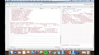
Emily Robinson walks through exploratory data analysis on the 2017 Kaggle Data Science survey using tidyverse packages. She shows how to read CSV files with readr, handle missing data, reshape with tidyr, and build charts with ggplot2, emphasizing reproducible code and clear visualizations.
Chapters
Hi everyone, my name is Emily Robinson and I'll be walking you through today some lesser known stars, the tidyverse. So first, a little bit about me. I come from a background in the social sciences, so in both my undergraduate and graduate studies I focus on learning, psychology, statistics, economics, and doing in person experiments. I've been using R for about seven years all through my studies. I was fortunate enough to go to Rice University when Hadley Wickham was teaching there, and Hadley's someone I'll talk about a little later in this talk if you're not familiar with that name. But he's a really great R programmer and teacher and I'm now a data scientist at datacamp. I work on the growth team here, focusing especially on building our AB testing or online experimentation system. And I came here from Etsy, where I worked with the search team, to similarly do lots of online experiments at Etsy, which is an E commerce company. So I have a couple goals for this talk. The first is to keep you hip to the lingo. So for those of you who are new to R in general, or maybe have been using R for a while, but haven't really gotten into the tidyverse. R maybe aren't quite sure what it is, or you think you know, but you're not sure why you should learn it, this talk should be really helpful for you. And the second is to stop you from throwing your computer away in frustration, because we all have those times where we know exactly what we want to do, but we just can't figure out the code to do it. Or maybe we figure out the code, but it's 50 lines long. And I'm going to help prevent this by teaching you some useful functions that will make your workflow a lot easier. So some of these functions come from packages you already may be familiar with if you've tried out the tidyverse, but others may be from packages you've never really heard of or didn't realize where they would be useful. And finally, I'm going to point you to some resources. So at the end of the talk I'm going to show you where you can go to learn more about the tidyverse, as hopefully I convinced you by then that it's a really worthwhile set of packages. It can help you in your R programming a lot. So what is this tidyverse? The official definition is it's a coherent system of packages for data manipulation, exploration and visualization that share a common design philosophy. So what does that mean exactly? Well, this is an overview of the tidyverse ecosystem. So we See different steps in the data analysis process here, such as importing your data, transforming it, communicating, and around those are the packages that help you do that. So, for example, to help transform your data, there's a stringr package which really helps you work with strings or the forecast package for categorical data. And so by sharing this common design philosophy, it makes it a lot easier to go across these different steps in a very smooth workflow. Now, if you have been around R for a little while, you might have heard of something called the Hadley verse, or even if you haven't, you know, the tidyverse functions that are packages that are probably best well known are ggplot2 and dplyr, and those were created by Hadley Wickham. So is the tidyverse just really like Hadley's set of packages? And the answer is absolutely not. Tidyverse does Not the Hadleyverse. So these are some of the great packages that make up the tidyverse, and these are the people behind them. In some cases, they're the original creators of the packages. In other cases, they're the current maintainers or they're very prominent contributors without whom the package wouldn't be what it is today. So I want to emphasize that the tidyverse, just as it's an ecosystem of packages, it's really an ecosystem of people who've helped support it, support it, and really make it thrive. And the main part of this talk, I'm going to actually be doing a live coding demo. So, so I, you know, I will preface this with this is data I have seen before, and I've, you know, sort of played around with it and run this code. But I want to show basically, okay, how would I approach an exploratory analysis of data and how, how did the tidyverse help me do it? And the data I'll be using is kaggle's State of Data Science and Machine Learning Survey. So actually now there is a new one out. This One is from 2017. So I got over 16,000 responses. It was sent out to people who are aspiring and practicing data scientists, but also, you know, machine learning engineers, business analysts, et cetera, kind of anyone who, you know is either in or wants to be in the data science and machine learning ecosphere. So I'm going to go ahead and switch over to R so we can start doing this analysis. All right, so I start off with this R project I've created. And, you know, the first step I always do is I'm a compulsive saver. So I'm going to go ahead and Save this. So I'll just call it tidyverse Webinar and. Oh, it already exists. Oh, yeah, I'll just replace it. Okay, so our first step whenever we're doing analysis is we need to read in the data. In this case, I actually have the data in a CSV. So, you know, if you've been around R for a while, you might be used to using just. Of course, read CSV. That's the way you read CSV. So read CSV. And my CSV is called MultipleChoiceResponses CSV. And first of, let's give that a go. So if I go ahead and I got to put it in my R file. There we go. So the first thing we notice is that it is taking a little while. Okay. But it eventually ran, and now I have a tidyverse person. So let's go ahead and load up the tidyverse package and I'll just put that up top. All right. So you notice we didn't need the tidyverse package for read CSV. That just comes built in with R, but we're going to need it for some other functions. So, you know, the first thing we might want to do is to count DNA's in a column. So it's really good to understand if you have missing data. So let's go ahead and just do it for one column. So if I want to do it for one column, one way might be to use the verb summarize. So here, what that's saying is, okay, take all this data and summarize it into an overall number. So in this case, I can do what's called sum is na. So sumisna works because IS NA transforms a variable into true or false based on whether or not it is na. And then by summing up these true and falses, true corresponds to 1, false to 0, and so I can know how many are NA. So I'll go ahead and run this and we see. Oh, okay, great. It doesn't seem like there are any NAs for this. That's really good news. Let's try this out for every column, though. So if I wanted to expand it, how would I see. Okay, I picked one column country. How would I see it for all the different columns? So now I'm gonna again, I'll take my data set. I'll use my favorite thing, pipe. So here, you know, what I'm doing is I'm passing the data set into the next argument, and I'm going to use per. And per is a great package that allows you to, you know, Apply a function to multiple columns, for example, in your data frame. So in this case, I'm going to use that function. Sum is na. I use this little tilde here. And then the other part of the code syntax is the dot. And so the dot here is representing basically every column and the tilde is essentially. All right, here's my formula. Sum is NA that I want you to apply to every column. And finally, you know, I'm using per map. I put this underscore DF because what I want back here is a data frame. So, so let me check that out now. All right, so if I run that PER is not found. There we go. I think I spelled it wrong. All right. And I didn't do the double colons. Yes. So I do the double colons. All right, that's cool. So now I can see this is, you know, looks like good news, right? All right, gender selection, country employment status, student status, those all have no NAs. But you should always be a little careful here of. Is this too good too be true? So let's take a look at one of these variables in this case, student status. So I take my data set and I pipe it to count. And count is really great because it's just a replacement for a group by and a summarize and getting you how many entries does each type in this column have? So if I look at counting student status, we see, all right, we see, yes, in student status, 981 times. No, 299 times. And then. Oh dear. We can see now that what's happened is that we have these empty strings that R doesn't recognize is equivalent in R to na, but in fact is. And that's. Actually, most people apparently didn't respond to this question. So what we want to do is we can use a function called NAIF to change those empty strings into na. So what we would do here is we would do this. We pipe it to naiif empty string. We run that again, we see. Okay, it's a little bit slow here. But right now that's because it's going across all different types of columns. And in any of the columns when it sees an empty string and we'll change that to an A. So if we wanted to modify our data set. So right here, if I looked now, let's say I did multiple choice response. And then I once again did counting the student status. You know, I don't. I didn't change anything. So the pipe isn't modifying the original data set. So I could do this in two ways. One way would be to reassign the data set to itself. So now if I do that, I run it, I try to count student status again. We see, oh, great, I fixed it. It's now in a. But you know, the other option here is we can use a different kind of pipe that will be equivalent. So instead we have the. We have two arrows in there and that's a reassignment pipe. So now it will change itself. So those two things I've just written are equivalent. And that's one way you can do to change something when you want to change your original data set rather than doing this arrow and basically reassigning it to itself. It's a little, you know, shorter code to just write this reassignment pipe. Okay, so now let's go back and we'll count the NA's again. So I'll go back, I'll copy my code for the permapdf and let's see if we've gotten any better. And yeah, look at that. So now we've got a really nice data set where we see. All right, it was too good to be true. Gender, select country, especially student status. They all do actually have nas. Now, how could we have avoided all of this in the first place? And a really good way is to use instead readr functions readcsv. So I'll try that now. And what, you know, and readr is basically the tidyverse way of reading in file. So if I, you know, also read in CSV again, let's see. All right, so the first thing we notice is one, it was a lot faster, but, you know, on the downside, it didn't have, you know, it says there were some problems. So we see. All right, what, you know, what are all these things? See problems for more details. So let's try out problems. So we'll wrap problems around our new variable multiple choice response responses and we'll see, all right, what we get back here is 31 rows. And each row it gives you actually a column that's called row, which is a row number, the column and the problem. So it's saying, all right, I expected there to be no trailing characters in the learning category online courses column on row 1344. But actually I see 0.5, you know, in this file. And these files will always be the same. So what's happening here is why one of the reasons readcsv is so fast is because it uses the first thousand rows to guess what the column type is. And in this case, it guessed Wrong because what happened was the first thousand rows of, you know, these columns might have or only had, you know, whole numbers or integers. But actually it is the case that sometimes people answered just 0.5. So how we can correct that is let's redo this. And now when we read the CSV we'll use the argument guessmax and guessmax. What it does is it says all right, instead of doing the default guessmax is going to be 1000, we're going to just have it know guess what type the column is based on, you know, all the rows. So here N row, you know, multiple choice, responsive. I look at that, 16,000. So that's what, how many rows it's going to use to guess. So if we run this again. All right, great. So we see it's still pretty fast and it didn't have any problems this time. So let's go on to the next step. Let's actually examine our data set now. Right. You've probably been sitting there and thinking okay, what. But you know, you talked about country and student status, but what does it actually look like? So you know, one way is you could just. Alright, what are even the columns that I have here? So if we look at those. Okay, multiple choice responses. All right, wow. So we see there were a lot, a lot of responses of columns here. So if I go all the way to the end, there's 228. Okay, this isn't a very helpful way to first look at it. So one thing I like to do is use a package called skimr, which comes from our open sci and specifically its function skim. So this is especially useful if you have numeric data. So I'm going to select all my numeric columns with the dplyr function selectif. So sort of as it sounds like it's saying all right, select columns if you know this condition inside is true. And in this case I'm giving it the condition that the color column is dot numeric. So now we'll use the skim our function skim, run that and great. So now we get lots of summary metrics for our variables. And one thing that is really nice here is that we have the missing data which I talked about before was important. We have the mean, the standard deviation. But actually probably my favorite feature is we have these little histograms and so it's really nice to get a quick view of your data. So one thing we can see is all right, learning self taught. You know, it seems like this in general has like a much Higher has a bigger range, and like, on average is higher, which we can see. All right, if we look at the 50th percentile, it's 30 here versus in some case it was zero in other columns. So it's a really nice way to just like, quickly look at your data. And it's also helpful because it's pointing out some problems. So if we look at the age variable, we see that the minimum number is 0 and the maximum is 100. Well, okay, that is, you know, we're not having people who are zero, and we're very likely no one was actually 100 who was taking this survey. So this is telling us, all right, we probably have some data quality issues that we would want to clean up, but for now, let's keep going. And another thing that I find really useful is getting the number of distinct answers for every question. So if we go back to our new function per mapdf, what we can do is same kind of formula. We do that tilde, we do the function ndistinct and we put the little dot in it. And ndistinct here is short for length, unique. And basically, so it's saying, all right, get all the. Make a vector of just the unique entries and. And then get me the length of that. So the number of unique. So indistinct is just a shorter way of doing that. So if we run this again, we get this data set back. That's one row, 228 columns. So the same number of columns as our original data set, but now only one row and it's summarized it. So here we see that, okay, gender has five options, right? Gender is not binary. It's not only, you know, two for male, female and radi three for other. We see country has 53 responses, employment status seven, etc. So, okay, this is sort of helpful, but really, this data is probably best not viewed in this really wide format, but actually in a long format. So we can do things like see which columns had the most distinct answers. So let's copy what we already did, and we're going to add onto it a tidyr function gather. And so tidyr is about reshaping your data. So, you know, there's a joke, it's very popular Twitter memes about how hard gather and spread, which are the two main tidyr functions, can be to remember their syntax. So don't feel bad if you have that happen to you. But basically, you know, this one is fairly straightforward. The two arguments we're going to give it are the two names of our new columns. So we're going to have it be question and num distinct answers. So if I look at what that looks like, we can see all the column names have gone into this new column question and all of the data entries have gone into the new column num distinct answers. So let's answer that question I just had. All right, so let me arrange the data in descending order by num distinct answers. And this again is going to get us, okay, what are the columns or questions that have the most distinct answers? All right, and we see that, you know, we have these little select columns. So work method select, learning platform select, etc. And this is pretty surprising that it has work method select has 6191. Remember, there are only a little over 16,000 people taking the survey in the first place. So let's try to figure out why does this have so many to say answers. So we'll go back and use the count function, which is really honestly like one of my favorite fairly simple, but function I use all the time. And let's count the work method select column. And the nice thing about count is you can give it this extra argument sort. And I'm going to say sort equals true. And this saves me from afterwards having to arrange it. So it's going to give it back to me already sorted. So let's see what the different work methods are. Okay. Okay, so we see NA seems to be the most popular data visualization other. But then we notice in this row that there are two methods that are separated by a comma. So if I keep looking, we see this happening over and over and based off of the column name. What's happening here is that people, it's a multiple selection option. So basically someone could choose maybe they only use one method, but maybe they use two, then they put both, you know, three, etc. So we're going to want to tidy this data and separate that out. So how I would do this is let's go ahead and just select the work methods column because that's all we're going to be focusing on right now. So work method select. Great. We just have this column. Let's filter for when it's not na. So a nice trick here is the exclamation point. And the exclamation point, right, is just says basically not. So exclamation point is not an A. Workmethodselect by filtering for that, we're selecting for when it's not an A. And then we're gonna do a mutate to create a new column workmethod. And we're gonna create it by splitting the work method select column on the comma. So let's see what that looks like. Okay, so we still have our original column work method select, and now we have this new column work method, and it's what's known as a list column. So we could see, all right, here, it's a list, a character list of length 5 or a list of length 12. And if we go back, we see. All right, Indeed, this had 1, 2, 3, 4, 5 answers that someone selected. So now it's separated out into lists. But this is still not very helpful. So our next step is going to be to unnest this data. So let's go ahead and copy this code again. And we're going to pipe it to the function unnest. And unnest says, all right, so I will give me a column and I will. Basically, it's a list column and I will split it out, make it a lot longer. So, so let's un nest it, select just the work method column, and see what that looks like. All right, so one thing to notice here is, wow, so there's now 59,000 rows, right? Compared to our old thing was like 7,000 after we took out the NA. And again, what's happening here is that first entry in the list column, which was five entries long, is now five different rows. And so it's become a much longer data set. And that's how we can use the un nesting to get that. And I'm just going to go ahead and save this as unnested work methods. Now. There's actually another way to do it that I only recently learned about. So instead of doing this, doing a string split and unnest, we can actually use a function called separate rows. So separate rows. Again, it takes that. It's very similar syntax to string split. So I take the column that I want to separate, and I take what do I want to separate it on? A comma and unknown comma. Right. So here I actually have to specify specifically that the comma is for the argument sep. And when I run that. Cool. So we see here again, we get these 59,000. So it's doing the same thing just a little bit more succinctly. So this is a really nice function that as it sounds like, right. It separates your column into rows using what you choose to separate it by. All right, so what kind of questions would I answer with now that I've parsed it out? I have Tidier data. Well, one just might be. What are the most frequent work methods? So if I go, if I use my unnested work methods that I created earlier and I count work method sort equals true. Let's take a look at what are the most popular ones. All right, so we see that data visualization, logistic regression and cross validation are coming out on top. And so these are also very like classic methods of data science and machine learning. So if I go to some of the least used, we see like Gans, we see Markov logic, evolutionary approaches. So it's kind of a nice reminder that, you know, all right, the basics are still really important, but even nicer than a table is a graph. So let's make a graph. So we'll copy our code here. So we'll do the counting of our unnested work methods, and then we're going to pipe it to ggplot and we're just going to make a simple bar chart here. So we're going to put work method on the X axis, N on the Y axis. We're going to use Geocoll. And then we're going to do a coordinate flip. Yeah. And let's take a look. All right, so now we've graphed our data here. I've done a coordinate flip because let's say if I take it away. All right, so now you can't read anything. Right. So the problem here is that all the text runs into each other. So that's why I flipped the coordinates around. Around. So now we see. Okay, you know, this is kind of useful. And I can still see that our data visualization looks like it's the top. You know, collaborative filtering doesn't have a lot of people. Gans really doesn't. But again, it's not as useful as if it was sorted. So what I'm going to do here is use a function called factor underscore, reorder. So I just copy all the code that I have, but now I change the X. So I change it to fctreorder, work method comma N. And I'm going to show you what this does and then explain it. All right, cool. So now we see that the access is ordered. And so what that was doing is it was saying take this column work method and reorder it by this other column N. And now that, that is what's going to be the exit that reordering shows up on our graph. And so it's much easier to read now and see that. Okay, here we go. We can just read from top to bottom, Gans is the least popular data visualization the most. All right, so let's move on to a different column now and look at the find all the columns about work challenges. So, you know, if we go back up and we see our column names, one thing we notice is we have a bunch of columns that are called work challenge frequency, something Work challenge frequency politics, Work challenge frequency, unused results. So let's take a look at all of those columns. And so how I do this is I'm going to use a select helper function contains. So I can actually select all the columns that contain the words work challenge frequency. So if I just take a look at that. Right, okay. Work challenge frequency, unused results, etc. We see we have the same number of rows now, only 22 columns because we just picked those with that had work challenge frequency in the name. So now that we've done that, let's go back to our trusty gather. We're going to put it make two new columns, question and response. Let's take a look at what that does. So now we see, oh wow, we have a lot more rows, but what we have is that we've made it a long data set instead of a wide one. So the question column has all the fun column names and the response of the responses. Now here again we notice a lot of them are in a. So let's go ahead and filter that out same way we did before. And now finally, let's make the question column a little easier to read. So something that's a bit annoying here, right, is they're all going to have work challenge frequency in it when we know that we selected the column name specifically to have that. So we can actually go ahead and remove that. So we're going to mutate the question column and use the stringr function str replace or actually str remove and this will remove the given string from a column. So if we can go ahead and remove work challenge frequency from the question column. And here we go. So now the question is just politics. It no longer says work challenge frequency. So I'm going to go ahead and save that as the work challenges data set. So now let's, you know, make this. So if we look at this now, all right, so we can see there are some different responses. So if we go ahead and we count the response, all right, there are four different responses that people can give most of the time, often, rarely, and so sometimes. So let's go ahead and dichotomize this variable. So this will make it A lot easier to show on one graph. So we're going to look at what are the percent of people considering it a work challenge, a problem, you know, and I'm going to say, all right, if they encounter it often or most of the time, that's a big problem. Rarely or sometimes not as much. So we'll take our work challenges data and we're going to change response to be 01 variable. So we're going to say, okay, response equals. If response is in most of the time or often, then it's going to be one else it should be zero. So now if we look at it, we say, all right, our response variable is 01. And the percent in percent is a really handy trick for if you, instead of doing like, you know, the other option might be like, response equal equals most of the time or response equals often or et cetera, you know, forever and ever until you die. Percent in, you can just list all the different responses you want it to match. So now we're going to go ahead and we're going to group by, you know, the question, and then we're going to summarize what percent of people think that something is a problem. And we're going to get that by just getting the mean of the response because again, we're saying, all right, if it's one, they consider it a problem, if it's zero, they don't. So we'll go ahead and do that. Okay. And now, because we've summarized our data set, we now only have one row per question. And we see that clarity, data access, data funds, etc. So again, this is probably more useful on a graph. So let's go ahead and graph it so we can save this first as a new data set. So we'll call it a percent problem work challenge, and then we'll take that, have that be our data set. We're going to graph. We only have two columns here. So let's put the question on the x axis and the, you know, the percent I consider a problem on the Y, we're just going to try out a point just to change it up from a bar chart and again, flip the coordinates. Okay, so now this is a little bit messy, right? We have the same problem we did before, so let's solve it the same way. So I'm going to just copy this code. I'm going to now surround question with factory order. So just like we did last time, reorder the question column by the percentage, I consider it a problem and try it again. All right? So now this is much more nicely done, but we want to. If we look at the x axis here now we see. All right, well, one issue here is that this is a percentage, but it doesn't have, you know, it's some 0.5, 0.6. Wouldn't it be nicer if it was 50, 50%, 60% instead? So we can use the function here, scale Y continuous and labels equals scales, percent. Now, I always get a little confused. It is, you know, the scale Y continuous, not scale X continuous, even though on this final resulting graph, percent problem is now on the Y axis or on the X axis. Excuse me. You know, and so it's a little funky here, and I never quite get it right. But, you know, if you don't get right, just try both of them. So in this case, all right, we can see now that we fixed it, and we can see, all right, 50% or 60% problem. And our final step is let's make these labels a little nicer. So, you know, our old label was, you know, just a percent problem, right? It just defaults, of course, to, you know, what the, you know, aesthetics you fed it in were. So you can use the labs, you know, we add labs to our gdplot. So we'll, let's say, you know, okay, X equals question, Y equals percentage. Encountering challenge frequently, and voila. So now we have a much more nicely labeled graph. All right, so now I'm going to return a little bit to the presentation to, to kind of wrap things up a bit. So let's go ahead and play that again. Okay, so your final step when you're doing this sort of thing is to try something cool and new. But what's one thing that can happen? Well, you can just have no idea what you're doing. So the problem could be that you're trying something new, but you just, like, you can't figure out how to figure this out, and where do you go and get help? So one solution is to make a minimum reproducible example, and that stands for it's all about letting someone else help you. So when you have a question, make it as easy as possible for someone else to figure out what your problem is and give you a solution. And you can do this with the Tibble package and the Reprex package. So TBL package is good because it has this function called Tribble. So sometimes you're running into a problem on a really complicated data set and you don't want, you know, you either. Maybe you can't give someone that data Set right? Or, you know, what are you going to do? Upload a CSV to stack overflow. So how can you show someone your problem? So triple is how I always dreamed of making toy data sets. So it does it on a row by row basis. So what we can see here is that what we have is little tildes in front of what are going to be our column names. So dates, a B test, a B variant we have, then we enter. All right, so what are some example rows? Here's the test, the a B test, the variant, and the percent with event. So this was actually sort of a real example for when I was running into a problem. And this was type that it was. So. But before we post it on some kind of website, we can use the Reprex package to find any problems. And reprex stands for reproducible example. And this is a great gift from Nick Tierney. And what it's showing you here is reprex, you know, when you copy your code and then you run the reprex function, it will run that code basically in a new and clean R session. And you can see what would happen. It's like, oh no, we have these errors, couldn't find the function ggplot or vismus. And if you look back at your code you're like, oh, of course, I never loaded the libraries in this chunk of code. And so maybe you'd loaded it previously in your R session, which is why it worked for you, but it wouldn't work for anyone just running this exact code. So once you've done this with Reprex, you can then use it to post your question or your issue. So Reprex makes it really easy to post even the graphs output. So we can see here that now Nick, he fixed his problem and he was able to submit an issue on GitHub, or you can put it on Stack Overflow or the R community site, or really anywhere that supports Markdown. So just as a review, here are some of the functions that we went over. So, so we talked about mathdf, naf Selectif, scim, Unnest, and just there's a really nice host of different functions that you can use, maybe from packages you've never heard of, but in some cases dplyr is where you get selectif and a lot of people who use dplyr may not know that one. So as promised, here's a lot of resources that you can go to to learn more about the tidyverse. Edit different functions. So I have to recommend Hadley Wickham and Garrett Grolemon's R for Data Science book, which is available for free online or you can buy a paper copy. This book is suitable for people totally new to R, but it can also be helpful even if you've been using R or even parts of the Tidyverse, if maybe you've never really gotten to understand tidy data or working with dates, you can just skip right ahead to that chapter where they'll walk you through how to use tidyverse functions for this. I'm a big fan of Twitter, so there's the rstats hashtag and this is a really great question to ask. Sort of what I call meta questions. So here's an example where I was saying, all right, does a method for this exist? So it's not a great question for like, look at my code. What's wrong with it? That's more of a kind of stack overflow question. But it's nice if like, oh, do you have a favorite package for doing X? Or does this package X exist? And in my case the answer was yes, you can set a theme globally. So Ilde Sessler here responds with tgtheme R package, which really helpfully they'd actually written a blog post about. So I was able to go ahead and use that and it solved my problem. The next thing I really like is RStudio has a bunch of cheat sheets. So. So for example, this is a cheat sheet for per. So Per, we saw the MAPDF function and that's often the function. The map functions are what people, what are called the apply functions are what people are kind of most familiar with Per with usually. But actually PER comes with a bunch of different functions. We see pluck and keep and flatten. So these are all really different great functions that can help you when you're working with lists. And of course, I couldn't fail to mention Data Camp. So. Right. I work here. Part of why I joined was that I'm a big fan of the data camp, you know, courses and projects and product. So here we just have. I searched tidyverse, we have just a couple we see right here, including introduction of the tidyverse, which is suitable for people who haven't done any program before. And we actually have a whole tidyverse fundamentals track with R. So my course is in here as well. Categorical data in the tidyverse. And it also has courses on communicating with data, working with data and modeling. So it's a really nice start. It's five courses long to start doing the tidyverse. If you never use datacamp before, this is what the interface looks like. So datacamp is also about interactive learning. Each course is about four hours long and it consists of usually like four chapters or so. Those chapters have maybe two, three, four minute videos, but most of your time is spent coding in a console. And so that way you can really quickly apply the skills that you've just learned on real problems. And a lot of the teachers use real interesting real world data sets. So in conclusion, the Tidyverse is, you know, really fun. One thing it has is lots of stickers. As you can see here, Christine Zhang is tweeting about. But what I also really love it is that there's a very friendly community and it can really help your workflow. So I hope I've shown you today how the Tidyverse functions can, you know, make exploratory analysis a little bit easier and less painful. And with that, thank you so much. You know, you can find find some of my writing, including basically a blog post version of this talk on hookedondata.org, my blog, and you can also follow me on Twitter obinsonyes. So usually occasionally I tweet about dog stuff, but mainly I'll either be tweeting or retweeting R or other data science resources. And thank you so much.
More from Richie

#359 My Best Friend is AI with Valerie Tiberius, Professor of Philosophy at University of Minnesota







How AI Agents Will Work While You Sleep | Ruslan Salakhutdinov, Professor at Carnegie Mellon

#358 How AI Agents Will Work While You Sleep | Ruslan Salakhutdinov, Professor at Carnegie Mellon

