Feature scaling improves gradient descent convergence. When features have different ranges, like house size in square feet versus number of bedrooms, the cost function creates elongated contours that slow down optimization. Rescaling features to comparable ranges makes contours circular and lets gradient descent converge much faster.
Chapters
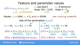
So, welcome back. Let's take a look at some techniques that will make gradient descent work much better. In this video, you see a technique called feature scaling that will enable gradient descent to run much faster. Let's start by taking a look at the relationship between the size of a feature, that is, how big are the numbers for that feature and the size of its associated parameter. As a concrete example, let's predict the price of a house using two features. X1 the size of the house and x2 the number of bedrooms. Let's say that x1 typically ranges from 300 to 2000 square feet, and x2 in the dataset ranges from 0 to 5 bedrooms. So for this example, x1 takes on a relatively large range of values and x2 takes on a relatively small range of values. Now, let's take an example of a house that has a size of 2,000 square feet, has five bedrooms and a price of 500K or $500,000. For this one training example, what do you think are reasonable values for the size of parameters W1 and W2? Well, let's look at one possible set of parameters. Say W1 is 50 and W2 is 0.1 and B is 50 for the purposes of discussion. So in this case, the estimated price in thousands of dollars is 100,000k here, plus 0.5k plus 50k, which is slightly over $100 million. So that's clearly very far from the actual price of $500,000. And so this is not a very good set of parameter choices for W1 and W2. Now let's take a look at another possibility. Say W1 and W2 were the other way around. W1 is 0.1 and W2 is 50, and B is still also 50. In this choice of W1 and W2, W1 is relatively small and W2 is relatively large. 50 is much bigger than 0.1. So here the predicted price is 0.1 times 2,055, 50. The first term becomes 200k, the second term becomes 250k and then plus 50. So this version of the model predicts a price of $500,000, which is a much more reasonable estimate and happens to be the same price as the true price of the house. So, hopefully you might notice that when a possible range of values of a feature is large, like the size in square feet, which goes all the way up to 2000, is more likely that a good model will learn to choose a relatively small parameter value like 0.1. Likewise, when the possible values of a feature are small like the number of bedrooms, then a reasonable value for its parameters will be relatively large, like 50. So how does this relate to gradient descent? Well, let's take a look at a scatter plot of the features where the size in square feet is the horizontal axis x1, and the number of bedrooms x2 is on the vertical axis. If you plot the training data, you notice that the horizontal axis is on a much larger scale or much larger range of values compared to the vertical axis. Next, let's look at how the const function might look in a cont4 plot. You might see a contour plot where the horizontal axis has a much narrower range, say between 0 and 1, whereas the vertical axis takes on much larger values, say between 10 and 100. So the contours form ovals or ellipses, and they're short on one side and longer on the other. And this is because a very small change to W one can have a very large impact on the estimated price and thus a very large impact on the cost J, because W1 tends to be multiplied by a very large number, the size in square feet. In contrast, it takes a much larger change in W2 in order to change the predictions much, and thus small changes to W2 don't change the cost function nearly as much. So where does this leave us? This is what might end up happening if you were to run gradient descent. If you were to use your training data as is, because the contours are so tall and skinny, gradient descent may end up bouncing back and forth for a long time before it can finally find its way to the global minimum. In situations like this, a useful thing to do is to scale the features. This means performing some transformation of your training data so that x1, say, might now range from 0 to 1 and x2 might also range from 0 to 1. So the data points now look more like this, and you might notice that the scale of the plot on the bottom is now quite different than the one on top. The key point is that the rescaled X1 and X2 are both now taking comparable ranges of values to each other. And if you run gradient descent on a cost function defined on this rescaled x1 and x2 using this transform data, then the contours will look more like this, more like circles and less tall and skinny. And gradient descents can find a much more direct path to the global minimum. So, to recap, when you have different features that take on very different ranges of values, it can cause gradient descent to run slowly. But rescaling the different features so they all take on comparable range of values, can speed up gradient descent significantly. How do you actually do this? Let's take a look at that in the next video.