Andrew Ng explains three ways to rescale features for machine learning: dividing by maximum, mean normalization, and Z-score normalization. He walks through examples like a feature ranging 300–2000 and shows why scaling features to roughly -1 to 1 speeds up gradient descent.
Questions this video answers
300 to 2000
0 to 5
600 (square feet)
2.3
450
Chapters
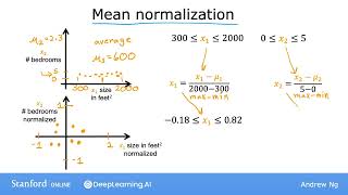
Let's look at how you can implement feature scaling to take features that take on very different ranges of values and scale them to have comparable ranges of value to each other. So how do you actually scale features? Well, if x1 ranges from 3 to 2000, one way to get a scale version of x1 is to take each original x1 value and divide by 2000 the maximum of the range. So the scale of x1 will range from 0.15 up to 1. Similarly, since x2 ranges from 0 to 5, you can calculate a scaled version of x2 by taking each original x2 and dividing by 5, which is again the maximum. So the scale x2 will now range from 0 to 1. So if you plot the scaled x1 and x2 on a graph, it might look like this. In addition to dividing by the maximum, you can also do what's called mean normalization. So what this looks like is you start with the original features and then you rescale them so that both of them are centered around zero. So whereas before they only had values greater than zero, now they have both negative and positive values, but maybe usually between negative 1 and plus 1. So to calculate the mean normalization of x1, first find the average, also called the mean of x1, on your training set, and let's call this mean mu1, with this being the Greek Alphabet mu. For example, you may find that the average of feature 1 mu1 is 600 square feet. So let's take each x1, subtract the mean mu1, and then let's divide by the difference 2000 minus 300, where 2000 is the maximum and 300 the minimum. And if you do this, you get the normalized x1 to range from minus 0.18 to 0.82. Similarly, to mean normalize x2, you can calculate the average of theta2, and for instance, mu2 may be 2.3. Then you can take each x2, subtract mu2 and divide by 5 minus 0. Again the max 5 minus the min, which is 0. The mean normalized x2 now ranges from minus 0.46 to 0.54. So if you plot the training data using the mean normalized x1 and x2, it might look like this. There's one last common rescaling method called Z score normalization. To implement Z score normalization, you need to calculate something called the standard deviation of each feature. If you don't know what the standard deviation is, don't worry about it. You won't need to know it. For this Class. Or if you've heard of the normal distribution, or the bell shaped curve, sometimes also called the Gaussian distribution, this is what the standard deviation for the normal distribution looks like. But if you haven't heard of this, you don't need to worry about that either. But if you do know what is the standard deviation, then to implement a Z score normalization, you first calculate the mean mu as well as the standard deviation, which is often denoted by the lowercase Greek Alphabet sigma of each feature. So, for instance, maybe feature 1 has a standard deviation of 450 and mean 600. Then to z score normalize x1, take each x1, subtract mu1 and then divide by the standard deviation, which I'm going to denote as Sigma 1. And what you might find is that the z score normalize x1 now ranges from minus 0.67 to 3.1. Similarly, if you calculate the second feature's standard deviation to be 1.4 and mean to be 2.3, then you can compute x2 minus mu2 divided by sigma2. And in this case, the z score normalized by x2 might now range from minus 1.6 to 1.9. So if you plot the training data on the normalized x1 and x2 on a graph, it might look like this. As a rule of thumb, when performing feature scaling, you might want to aim for getting the features to range from maybe anywhere around minus 1 to somewhere around 1 for each feature X. But these values minus 1 and 1 can be a little bit loose. So if the features range from -3 to 3 or -0.3 to 0.3, all of these are completely okay. So if you have a feature X1 that winds up being between 0 and 3, that's not a problem. And you can rescale it if you want. But if you don't rescale it, it should work okay, too. Or if you have a different feature x2 whose values are between -2 and 0.5, again, that's okay, no harm rescaling it, but it might be okay if you leave it alone as well. But if another feature like X3 here ranges from minus 100 to 100, then this takes on a very different range of values than something from around minus 1 to 1. So you're probably better off rescaling this feature x3 so that it ranges from something closer to minus 1 to 1. Similarly, if you have a feature x4 that takes on really small values, say between minus 0.001 and 0.001, then these values are so small that means you may want to rescale it as well. Finally, what if your feature x5, such as measurements of a hospital patient's body Temperature, ranges from 98.6 to 105 degrees Fahrenheit? In this case, these values are around 100, which is actually pretty large compared to other scale features. And this will actually cause gradient descent to run more slowly. So in this case, feature rescaling will likely help. There's almost never any harm to carrying out feature rescaling, so when in doubt, I encourage you to just carry it out. And that's it for feature scaling. With this little technique, you'll often be able to get gradient descent to run much faster. So that's feature scaling. And with or without feature scaling, when you run gradient descent, how can you know? How can you check if gradient descent is really working if it is finding you the global minimum or something close to it? In the next video, let's take a look at how to recognize if gradient descent is converging, and then in the video after that, this will lead to a discussion of how to choose a good learning rate for gradient descent.