#33 Machine Learning Specialization [Course 1, Week 3, Lesson 1]

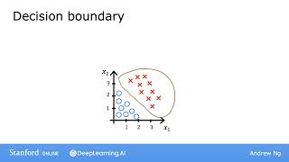
In the last video, you learned about the logistic regression model. Now let's take a look at the decision boundary to get a better sense of how logistic regression is computing its predictions. To recap, here's how the logistic regression model's outputs are computed in two steps. In the first step, you compute Z as W dot x plus B. Then you apply the sigmoid function G to this value z. And here again is the formula for the sigmoid function. Another way to write this is we can say F of X is equal to G, the sigmoid function, also called the logistic function, applied to W dot x plus b, where this is, of course, the value of z. And if you take the definition of the sigmoid function and plug in the definition of z, then you find that F of X is equal to this formula over here, one over one plus e to the negative Z, where Z is wx plus B. And you may remember we said in the previous video that we interpret this as the probability that Y is equal to 1 given x and with parameters W and B. And so this is going to be a number like maybe 0.7 or 0.3. Now, what if you want the learning algorithm to predict, is the value of Y going to be 0 or 1? Well, one thing you might do is set a threshold above which you predict Y is one, or you set Y hat prediction to be equal to one, and below which you might say Y hat, my prediction is going to be equal to zero. So a common choice would be to pick a threshold of 0.5, so that if F is greater than or equal to 0.5, then predict y is 1, and we write that prediction as y hat equals 1. Or if f is less than 0.5, then predict y Is 0, or in other words, the prediction Y hat is equal to zero. So now let's dive deeper into when the model would predict one. In other words, when is F greater than or equal to 0.5? We'll recall that F is just equal to G of Z. And so F is greater than OR equal to 0.5 whenever G of Z is greater than or equal to 0.5. But when is G of Z greater than or equal to 0.5? Well, here's a sigmoid function over here. And so G of Z is greater than or equal to 0.5 whenever z is greater than or equal to 0, right? That is, whenever z is on the right half of this axis. And finally, when is Z greater than or equal to 0? Well, z is equal to w dot x plus b, and so z is greater than or equal to 0 whenever w dot x plus b is greater than or equal to 0. So, to recap, what you've seen here is that the model predicts one whenever w dot x plus b is greater than or equal to zero. And conversely, when W dot x b is less than zero, the algorithm predicts Y is zero. So given this, let's now visualize how the model makes predictions. I'm going to take an example of a classification problem where you have two features, X1 and X2. Instead of just one feature, here's a training set where the little red crosses denote the positive examples and the little blue circles denote negative examples. So the red crosses corresponds to y equals 1 and the blue circles correspond to y 0. So the logistic regression model will make predictions using this function F of x equals G of Z, where Z is. Now, this expression over here, W1, X1 plus W2, X2B. Because we have two features, X1 and X2. And let's just say for this example that the value of the parameters are W1 equals 1, W2 equals 1, and B equals negative 3. And let's now take a look at how logistic regression makes predictions. In particular, let's figure out when wx plus B is greater than or equal to zero and when wx plus b is less than zero. To figure that out, there's a very interesting line to look at, which is when wx plus b is exactly equal to zero. It turns out that this line is also called the decision boundary, because that's the line where you're just almost neutral about whether y is 0 or y is 1. Now, for the values of the parameters w1, w2, and b that we had written down above, this decision boundary is just x1, x2 minus 3. And so when is x1 plus x2 minus 3 equal to 0? Well, that will correspond to the line x1, x2 equals 3, and that is this line shown over here. And so this line turns out to be the decision boundary where if the features x are to the right of this line, logistic regression would predict one, and to the left of this line, logistic regression would predict zero. In other words, what we have just visualized is the decision boundary for logistic regression when the parameters W1, W2, and B are 1, 1, and negative 3. Of course, if you had a different choice of the parameters, the decision boundary would be a different line. Now, let's look at a more complex example where the Decision boundary is no longer a straight line as before. Crosses denote the class y equals 1, and the little circles denote the class y equals 0. Earlier last week you saw how to use polynomials in linear regression, and you can do the same in logistic regression. So let's set z to be W1x1 squared plus W2x2 squared plus B. With this choice of features, polynomial features, into a logistic regression. So F which equals G is now g of this expression over here. And let's say that we end up choosing W1 and W2 to be 1 and B to be negative 1. So Z is equal to 1 times x 1 squared plus 1 times x 2 squared minus 1. And the decision boundary as before will correspond to when z is equal to 0. And so this expression will be equal to 0 when x1 squared plus x2 squared is equal to 1. And if you plot on the diagram on the left, the curve corresponding to x1 squared plus x2 squared equals 1. This turns out to be this circle. When x1 squared plus x2 squared is greater than or equal to 1, that's this area outside the circle. And that's when you predict y to be 1. Conversely, when x1 squared plus x2 squared is less than 1, that's this area inside the circle. And that's when you would predict Y to be zero. So can we come up with even more complex decision boundaries than these? Yes, you can. You can do so by having even higher order polynomial terms, say z is w1 x1 plus w2 x2 plus w3 x1 squared plus w4 x1 x2 plus w5 x2 squared. Then it's possible you can get even more complex decision boundaries. The model can define decision boundaries such as this example, an ellipse that's like this, or with a different choice of the parameters, you can even get more complex decision boundaries which can look like functions that maybe look like that. So this is an example of an even more complex decision boundary than the ones we've seen previously. And this implementation of logistic regression will Predict y equals 1 inside this shape, and outside the shape will predict Y equals zero. So with these polynomial features, you can get very complex decision boundaries. In other words, logistic regression can learn to fit pretty complex data. Although if you were to not include any of these higher order polynomials, so if the only features you use are x1, x2, x3 and so on, then the decision boundary for logistic regression will always be linear, will always be a straight line. In the upcoming optional lab, you also get to see the code implementation of the decision boundary. In the example in the lab, there will be two features, so you can see the decision boundary as a line. So with these visualization, I hope that you now have a sense of the range of possible models you can get with logistic regression. Now that you've seen what F of x can potentially compute, let's take a look at how you can actually train a logistic regression model. We'll start by looking at the cost function for logistic regression, and after that figure out how to apply gradient descent to it. Let's go on to the next video.