Andrew Ng derives the gradient descent update rules for logistic regression, showing how they resemble linear regression but use sigmoid activation. He covers simultaneous parameter updates, vectorization, and feature scaling to speed convergence, then points to Scikit-Learn for practical implementation.
Chapters
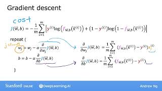
To fit the parameters of a logistic regression model, we're going to try to find the values of the parameters W and B that minimize the cost function j of W and B. And we'll again apply gradient descent to do this. Let's take a look at how. In this video we'll focus on how to find a good choice of the parameters W and B. After you've done so, if you give the model a new input X, say a new patient at the hospital with a certain tumor size and age that needs a diagnosis, the model can then make a prediction, or it can try to estimate the probability that the label Y is one. The algorithm you can use to minimize the cost function is gradient descent. Here again is the cost function. And so if you want to minimize the cost J as a function of W and B, well, here's the usual gradient descent algorithm where you repeatedly update each parameter as the O value minus alpha. The learning rate times this derivative term. Let's take a look at the derivative of j with respect to wj. This term up on top here, where as usual, j goes from 1 through n, where n is the number of features. If someone were to apply the rules of calculus, you can show that the derivative with respect to wj of the cost function capital J is equal to this expression over here. It's 1 over m times the sum from 1 through m of this error term, that is f minus the label y times xj here. This xij is the j feature of training example I. Now let's also look at the derivative of j with respect to the parameter B. It turns out to be this expression over here. And it's quite similar to the expression above, except that it is not multiplied by this X superscript I subscript j at the end. So, just as a reminder, similar to what you saw for linear regression, the way to carry out these updates is to use simultaneous updates, meaning that you would first compute the right hand side for all of these updates and then simultaneously overwrite all the values on the left at the same time. So let me take these derivative expressions here and plug them into these terms here. This gives you gradient descent for logistic regression. Now, one funny thing you might be wondering is, huh, that's weird. These two equations look exactly like the algorithm we had come up with previously for linear regression. So you might be wondering, is linear regression actually secretly the same as logistic regression? Well, even though these equations look the same, the reason that this is not linear regression is because the definition for the function F has changed in Linear regression F of x is this is wx plus b, but in logistic regression, F is defined to be the sigmoid function applied to wx plus b. So although the algorithm written looked the same for both linear regression and logistic regression, actually they're two very different algorithms because the definition for F is not the same. When we talked about gradient descent for linear regression previously, you saw how you can monitor gradient descent to make sure it converges. You can just apply the same method for logistic regression to make sure it also converges. I've written out these updates as if you're updating the parameters wj1 parameter at a time. Similar to the discussion on vectorized implementations of linear regression, you can also use vectorization to make gradient descent run faster for logistic regression. I won't dive into the details of the vectorized implementation in this video, but you can also learn more about it and see the code in the optional labs. So now you know how to implement gradient descent for logistic regression. You might also remember feature scaling when we were using linear regression where you saw how feature scaling, I.e. scaling all the features to take on similar ranges of values, say between negative one and plus one, how that can help gradient descent to converge faster. Feature scaling, applied the same way to scale the different features to take on similar ranges of values, can also speed up gradient descent for logistic regression. In the upcoming optional lab, you also see how the gradient for logistic regression can be calculated in code. This will be useful to look at because you also implement this in the practice lab at the end of this week. After you run gradient descent in this lab, there'll be a nice set of animated plots that show gradient descent in action. You see the sigmoid function, the contour plot of the cost, the 3D surface plot of the cost, and the learning curve all evolve as gradient descent runs. There will be another optional lab after that, which is short and sweet, but also very useful because I'll show you how to use the popular SciKit Learn Library to train the logistic regression model for classification. Many machine learning practitioners in many companies today use Scikit Learn regularly as part of their job, and so I hope you check out the SciKit Learn function as well and take a look at how that is used. So that's it. You now know how to implement logistic regression. This is a very powerful, very widely used learning algorithm and you now know how to get it to work yourself. Congratulations.