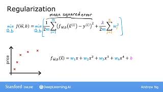
Andrew Ng explains how to add a penalty term to the cost function that discourages large parameter values and reduces overfitting. A tiny lambda leads to overfitting, an enormous one like 10^10 collapses the model to just the bias term, so you have to pick the right value.
Questions this video answers
Divide lambda times the sum of w_j^2 by 2m (i.e., use (lambda/(2m)) * sum_{j} w_j^2).
No — by convention the bias term b is not penalized (though some implementations may include it).
Lambda = 0 (no regularization) → can overfit; very large lambda (example given: 10^10) → underfit (parameters ≈ 0, model ≈ bias-only).
Chapters
In the last video, we saw that regularization tries to make the parameter values W1 through WN small to reduce overfitting. In this video, we'll build on that intuition and develop a modified cost function for your learning algorithm that you can use to actually apply regularization. Let's jump in. Recall this example from the previous video in which we saw that if you fit a quadratic function to this data, it gives a pretty good fit. But if you fit a very high order polynomial, you end up with a curve that overfits the data. But now consider the following. Suppose that you had a way to make the parameters W3 and W4 really, really small, say, close to zero. Here's what I mean. Let's say instead of minimizing this objective function, this is a cost function for linear regression. Let's say you were to modify the cost function and add to it 1000 times W3 squared plus 1000 times W4 squared. And here I'm just choosing 1000 because it's a big number, but any other really large number would be okay. So with this modified cost function, you'd in effect be penalizing the model if W3 and W4 are large. Because if you want to minimize this function, the only way to make this new cost function small is if w3 and w4 are both small, right? Because otherwise this 1000 times w3 squared and 1000 times w4 squared terms are going to be really, really big. So when you minimize this function, you're going to end up with W3 close to zero and W4 close to zero. So we're effectively nearly canceling out the effect of the features X cubed and x to the power of four and getting rid of these two terms over here. And if we do that, then we end up with a fit to the data that's much closer to the quadratic function, including maybe just tiny contributions from the features X cubed and x to the 4. And this is good because it's a much better fit to the data compared to if all the parameters could be large, and you end up with this wiggly quadratic function. More generally, here's the idea behind regularization. The idea is that if there are smaller values for the parameters, then that's a bit like having a simpler model, maybe one with fewer features, but which is therefore less prone to overfitting. On the last slide, we penalize, or we say we regularized only W3 and W4. But more generally, the way that regularization tends to be implemented is if you have a Lot of features, say 100 features. You may not know which are the most important features and which ones to penalize. So the way regularization is typically implemented is to penalize all of the features, or more precisely, you penalize all the WJ parameters. And it's possible to show that this will usually result in fitting a smoother, simpler, less wiggly function that's less prone to overfitting. So for this example, if you have data with 100 features for each host, it may be hard to pick in advance which features to include and which ones to exclude. So let's build a model that uses all 100 features. So you have these 100 parameters, W1 through W100, as well as the 101st parameter B. Because we don't know which of these parameters are going to be the important ones, let's penalize all of them a bit and shrink all of them by adding this new term lambda times the sum From j equals 1 through n, where n is 100, the number of features of wj squared. This value lambda here is the Greek Alphabet lambda and is also called a regularization parameter. So, similar to picking a learning rate alpha, you now also have to choose a number for lambda. Couple things I would like to point out. By convention, instead of using lambda times the sum of WJ squared, we also divide lambda by 2m, so that both the first and second terms here are scaled by 1, 2m. It turns out that by scaling both terms the same way, it becomes a little bit easier to choose a good value for lambda. And in particular, you find that even if your training set size grows, say you find more training examples, so M, the training set size is now bigger. The same value of lambda that you have picked previously is now also more likely to continue to work if you have this extra scaling by 2m. Also, by the way, by convention, we're not going to penalize the parameter B for being large. In practice, it makes very little difference whether you do or not. And some machine learning engineers, and actually some learning algorithm implementations, will also include lambda over 2m times the B squared term. But this makes very little difference in practice. And the more common convention which we'll use in this course is to regularize only the parameters w rather than the parameter b. So to summarize, in this modified cost function, we want to minimize the original cost, which is the mean squared error cost, plus additionally the second term, which is called the regularization term. And so this new cost function trades off two goals that you might have trying to minimize this first term encourages the algorithm to fit the training data well by minimizing the squared differences of the predictions and the actual values, and try to minimize the second term. The algorithm also tries to keep the parameters WJ small, which will tend to reduce overfitting. The value of lambda that you choose specifies the relative importance or the relative trade off or how you balance between these two goals. Let's take a look at what different values of lambda will cause your learning algorithm to do. Let's use the housing price prediction example using linear regression. So F is the linear regression model. If lambda was set to be zero, then you're not using the regularization term at all because the regularization term is multiplied by zero. And so if lambda was zero, you end up fitting this overly wiggly, overly complex curve and it overfits. So that was one extreme of if lambda was zero. Let's now look at the other extreme. If you set lambda to be a really, really, really large number, say lambda equals 10 to the power of 10, then you're placing a very heavy weight on this regularization term on the right. And the only way to minimize this is to be sure that all the values of W are pretty much very close to zero. So if lambda is very, very large, the learning algorithm will choose W1, W2, W3, and W4 to be extremely close to zero. And thus F is basically equal to B. And so the learning algorithm fits a horizontal straight line and underfits. To recap, if lambda is zero, this model will overfit. If lambda is enormous, like 10 to the power of 10, this model will underfit. And so what you want is some value of lambda that is in between that more appropriately balances these first and second terms of trading off, minimizing the mean squared error and keeping the parameters small. And when the value of lambda is not too small and not too large, but just right, then hopefully you end up able to fit a fourth order polynomial keeping all of these features, but with a function that looks like this. So that's how regularization works. When we talk about model selection later in the specialization, we'll also see a variety of ways to choose good values for lambda. In the next two videos, we'll flesh out how to apply regularization to linear regression and logistic regression and how to train these models with gradient descent. With that, you'll be able to avoid overfitting with both of these algorithms.