C4W1L07 One Layer of a Convolutional Net
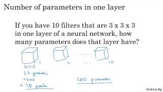
A convolutional layer takes an input volume, convolves it with multiple filters, adds bias, applies ReLU, and stacks the results. A 6×6×3 input becomes 4×4×2 output. Ten 3×3×3 filters create 280 total parameters, a count that doesn't change with input size.
Questions this video answers
Input: 6×6×3; Output: 4×4×2.
280 parameters (10 × (3×3×3 + 1) = 10 × 28).
F^[L] denotes filter size, P^[L] denotes padding, and S^[L] denotes stride.
Chapters
You're now ready to see how to build one layer of a convolutional neural network. Let's go through an example you've seen in the previous video. How to take a 3D volume and convolve it with say two different filters in order to get in this example, two different 4x4 outputs. So let's say convolving with the first filter gives this first 4x4 output, and convolving with this second filter gives a different 4x4 output. The final thing to turn this into a convolutional neural net layer is that for each of these we're going to add a bias. So this is going to be a row number. And with Python broadcasting, you kind of add the same number to every, you know, one of these 16 elements and then apply a non linearity which for illustration that says a relu nonlinearity. And this gives you a four by four output, right? After applying a bias and a nonlinearity. And then for this thing at the bottom as well, you add some different bias. Again this is a real number. So you add the same row number to all 16 numbers and then apply some non linearity, let's say a relu nonlinearity. And this gives you a different 4 by 4 output. Then same as we did before, if you take this and stack it up as follows, so you end up with a 4 by 4 by 2 output. Then this computation where you've gone from a 6 by 6 by 3 to a 4 by 4 by 4, this is one layer of a convolutional neural network. So to map this back to one layer of forward propagation in a standard neural network on a non convolutional neural network, remember that one step of forward prop was something like this, right? Z1 equals w1 times a0 and a0 was also equal to x, right? And then plus b1 and you apply the nonlinearity to get a1. So that's g of. So this input here in this analogy, this is a zero, this is X really. And these filters here displays a row similar to W1. And you remember during the convolution operation you're taking these 27 numbers or really well, 27 times two because you have two filters, we're taking all of these numbers and multiplying them. So you. So you're really computing a linear function to get this 4 by 4 matrix. So that 4 by 4 matrix, the output of the convolution operation that plays a role similar to W1 times A0 as really maybe the output of this 4x4 as well as that 4 by 4. And then the other thing you do is add the bias. So this thing here, before applying relu, this plays a role similar to Z. And then it's finally by applying the non linearity, you know, it's kind of this, I guess. So this output, right, plays a role. This really becomes your activation at the next layer. So this is how you go from a zero to to a one. That's first the linear operation and then the convolution has all these multiplied. So the convolution is really applying a linear operation and you add the biases and you apply a relu operation and you've gone from a six by six by three dimensional a zero through one layer of a neural network to I guess a four by four by two dimensional a, a one. So six by six by three has gone to four by four by two. And so that's one layer of a convolutional net. Now in this example we had two filters. So we had, you know, two features, if you will, which is why we wound up with an output 4 by 4 by 2. But if for example, we instead had 10 filters instead of 2, then we'd have wound up with a 4 x 4 x 10 dimensional output volume. Because we'd be taking 10 of these maps, not just two of them, and stacking them up to form a 4 x 4 x 10 output volume. And that's what a 1 would be. So to make sure you understand this, let's go through an exercise. Let's suppose you have 10 filters, not just two filters that are three by three by three. In one layer of a neural network. How many parameters does this layer have? Well, let's figure this out. Each filter is a 3 by 3 by 3 volume. So 3 by 3 by 3. So each filter has 27 parameters, right? So it's 27 numbers to be learned and then plus the bias. So that was the B parameter. So this gives you 28 parameters. And then if you imagine that on the previous slide, you know, we had drawn two filters. But now if you imagine that you actually have 10 of these, like 1, 2, 10 of these, then altogether you would have 28 times 10. So that would be 280 parameters. Notice one nice thing about this is that no matter how big the input image is, the input image could be 1,000 by 1,000 or 5,000 by 5,000. But the number of parameters you have still remains fixed as 280. And you can use these 10 filters to detect features you know, vertical edges, horizontal edges, maybe other fields, features anywhere, even in a very, very large image with just a very small number of parameters. So this is really one property of convolutional neural nets that makes them less prone to overfitting that you can, so long as you learn 10 feature detectors that work, you could apply this even to very large images. And the number of parameters still remains fixed and relatively small as 280. And in this example. All right, so to wrap up this video, let's just summarize the notation we're going to use to describe one layer, to describe a convolutional layer in a convolutional neural network. So layer L is a convolutional layer. I'm going to use F superscript square bracket L to denote the filter size. So previously we've been saying the filters are F by f, and now this superscript square bracket L just denotes that this is a filter size, is a F by F filter in layer L. And as usual, the super square bracket L is the notation we're using to refer to a particular layer L. Gonna use PL to denote the amount of padding. And again, the amount of padding can also be specified just by saying that you want a valid convolution, which means no padding, or a same convolution, which means you choose the padding so that the output size has the same height and width as the input size, and then going to use SL to denote the stride. Now, the input to this layer is going to be some dimension, it's going to be some N by n by number of channels in the previous layer. Now I'm going to modify this notation a little bit. I'm going to use superscript L minus 1 because that's the activation from the previous layer L minus 1 times NC of L1. And in the example so far we've been just using images with the same height and width. But in case the height and width might differ, I'm going to use superscript H and superscript W to denote the height and width of the input from the previous layer. So in layer L, the size of the volume will be nh by nw by nc with superscript, you know, square bracket l. It's just that in layer L, the input to this layer is whatever you had from the previous layer. So that's why you have l minus one there. And then the neural network, excuse me, this layer, and then this layer of the neural network will output, will itself output a volume. So, so that would be NH of L by NW of L by NC of L, that will be the size of the output. And so whereas we have previously said that the output volume size, or at least the height and width is given by this formula, you know, N + 2P + F + S + 1 and then take the floor of that or round it down. In this new notation, what we have is that the output volume that is in layer L is going to be the dimension from the previous layer, plus the padding we're using in this layer L minus the filter size, we're using this layer L and so on. And technically this is true for the height, right? So the height of the output volume is given by this and you can compute it with this formula on the right. And the same is true for the width as well. So if you cross out H and throw in W as well, then you know, the same formula with either the height or the width plugged in works for computing the height or width of the output volume. So that's how NHL -1 relates to NHL and NWL -1 relates to NWL. Now how about the number of channels? Where do those numbers come from? Let's take a look. If the output volume has this depth, well we know from the previous examples that that's equal to the number of filters we have in that layer, right? So we had two filters. The output volume was 4 by 4 by 2, was two dimensional. And if you had 10 filters, then the output volume was 4 by 4 by 10. So this the number of channels in the output volume, that's just the number of filters we're using in this layer of the neural network. Next, how about the size of each filter? Well, each filter is going to be FF by FL by one other number, right? So what is this last number? Well, we saw that you need to convolve a 6 by 6 by 3 image with a 3 by 3 by 3 filter. And so the number of channels in your filter must match the number of channels in your input. So this number should match that number, right? Which is why each filter is going to be FL by FL by N cl. And the output of this layer, after applying the biases and the nonlinearity is going to be the activations of this layer Al. And that we've already seen will be this dimension, right? The Al will be a 3D volume. That's NHL by NW, L by NC. Hello. And when you are using a vectorized implementation or you know, batch gradient descent or mini batch gradient descent, then you actually output Al, which is set of um, M activations. If you have M examples. So that will be M by NHL by NWL by ncl. Right. If say you're using batch gradient descent and in the programming exercises this will be the DEF dimension. This will be ordering of the variables and we have the index and the training examples first and then you know, these three variables next. How about the weights or the parameters or kind of the W parameter? Well, we saw already what the filter dimension is. So the filters are going to be FL by FL by NCL minus 1, but that's the dimension of one filter. How many filters do we have? Well, this is the total number of filters. So the weights really all of the filters put together will have dimension given by this times the total number of filters. Right? Because this last quantity is the number of filters in layer L. And then finally you have the bias parameters and you have one bias parameter, one real number for each filter. So you're going to have, you know, the bias will have this many variables. It's just a vector of this dimension. Although later on we'll see that in the code it'll be more convenient to represent it as a one by one by one by nc L dimensional, you know, four dimensional matrix or four dimensional tensor. So I know that was a lot of notation. Um, and this is the convention I'll use for the most part. I just want to mention in case you search online and look at open source code, there isn't a completely universal conven standard convention about the ordering of height, width and channels. So if you look on Source code on GitHub or read some of the open source implementations, you find that some authors use this order instead, where you first put the channel first and you sometimes see that ordering of the variables and in fact in some programming frameworks, actually in multiple programming frameworks, is actually a variable or a parameter. Whether you want to list the number of channels first or list the number of channels last when indexing into these volumes. And I think both of these conventions work okay so long as they are consistent. And unfortunately maybe this isn't. And unfortunately, maybe this is one piece of notation where there isn't consensus in the deep learning literature. But I'm gonna use this convention for these videos where we list, you know, height and then width and then the number of channels lost. So I know there was suddenly a lot of new notation to introduce. Uh, but you're thinking, wow, this is a lot of notation. How do I need to remember all of these? Don't worry about it, you don't need to remember all of this notation, and through this week's exercises, you become more familiar with it at that time. But the key point I hope you take away from this video is just how one layer of a convolutional neural network works. And the computations involved in taking the activations of one layer and and mapping that to the activations of the next layer. And next now that you know how one layer of a convolutional neural network works, let's stack a bunch of these together to actually form a deeper convolutional neural network. Let's go on to the next video to.










