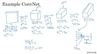
Lecture (Andrew Ng) giving a concrete example of a small convolutional neural network for image classification. Starts from a 39×39×3 input, walks through three convolutional layers (3×3 then two 5×5 layers) with specified strides, computes the resulting activation volumes (37×37×10 → 17×17×20 → 7×7×40), and shows flattening the final 7×7×40 volume to a 1960-length vector to feed a logistic/softmax output. Concludes with remarks that designers choose hyperparameters (filter size, stride, padding, number of filters) and that pooling and fully connected layers will be covered next.
Questions this video answers
39 × 39 × 3
3 × 3 (F1 = 3)
10 filters (NC1 = 10)
37 × 37 × 10
5 × 5 filters with stride 2 (F2 = 5, S2 = 2)
Chapters
In the last video, you saw the building blocks of a single layer of a single convolutional layer in a convnet. Now let's go through a concrete example of a deep convolutional neural network. And this will give you some practice with the notation that we introduced toward the end of the last video as well. Let's say you have an image and you want to do image classification or image recognition, where you want to take as input and image X and decide, is this a cat or not? 0 or 1. So it's a, you know, classification problem. So let's build a notional. Let's build an example of a confnet you could use for this task. Um, for the sake of this example, I'm gonna use a fairly small image. Let's say this image is 39 by 39 by 3. Uh, this choice just makes some of the numbers work out a bit better. And so nh in layer 0 will be equal to nw height and width I equal to 39. And the number of channels in layer 0 is equal to 3. Let's say the first layer uses a set of 3 by 3 filters to detect features. So f is equal to 3 already, f1 is equal to 3 because we're using 3 by 3 filters. And let's say we're using a stride of 1 and no padding. So using a same convolution, and let's say you have 10 filters, then the activations in this next layer of the neural network will be 37 by 37 by 10. And this 10 comes from the fact that you use 10 filters. And 37 comes from this formula. N plus 2Pminus F over S plus 1. Right? And I guess you have 39 plus 0 minus 3 over 1 plus 1. That's equal to 30. So that's why the output is 37 by 37. It's a valid convolution. And that's the output size. So in our notation you would have NH1 equals NW1 equals 37 and NC1 is equal to 10. So NC1. This is also equal to the number of filters from the first layer. And so this becomes the dimension of the activation at the first layer. Let's say you now have another convolutional layer. And let's say this time you use 5 by 5 filters. So in our notation, F2 at the next layer of neural network is equal to five. Um, and let's say you use a stride of two this time and maybe you have, uh, no padding. And say 20 filters. So then the output of this will be another volume. This time it'll be 17 by 17 by 20. Notice that because you're now using a stride of two, the dimension has shrunk much faster, right? 37 by 37 has gone down in size by slightly more than a factor of 2 to 17 by 17. And because you're using 20 filters, the number of channels now is 20. So this activation A2 would be that dimension. And so NH2 equals NW2 equals 17 and NC2 equals 20. All right, let's apply one last convolutional layer. So let's say that you use a five by five filter again and again a stride of two. So if you do that, I'll skip the map, but you end up with a 7 by 7. And let's say you use 40 filters, no padding, 40 filters, you end up with 7 by 7 by 40. So now what you've done is taken your 39 by 39 by 3 input image and computed, you know, 7 by 7 by 40 features for this image. And then finally, what's commonly done is if you take this 7 by 7 by 40, 7 times 7 times 40 is actually 1960. And so we can do is take this volume and flatten it or unroll it into, you know, just 100 into 1960 units, right? Just as a, as a, flatten it out into a vector and then feed this to a logistic regression unit or a softmax unit, depending on whether you're trying to recognize cat, no cat, or trying to recognize any one of k different objects. And then just have this give the final output, the final predicted output for the neural network network. And so just be clear, this last step is just taking all of these numbers, 100 or 1960 numbers, and unrolling them into a very long vector. So then you just have one long vector that you can feed into softmax into logistic regression in order to make a prediction for the final output. So this would be a pretty, you know, typical example of a confnent. A lot of the work in designing a convolutional neural net is selecting hyperparameters like these, deciding what's the filter size, what's the stride, what's the padding, and how many filters to use. And both later this week as well as next week will give some suggestions and some guidelines for how to make these choices. But for now, maybe one thing to take away from this is that as you go deeper in a neural network, typically you start off with larger images, 39 39. And then the height and width will, you know, stay the same for a while and, and gradually trend down as you go deeper into neural networks. It's gone from 39 to 37 to 17 to 40. Excuse me, this has gone from 39 to 37 to 17to7, whereas the number of channels will generally increase, has gone from 3 to 10 to 20 to 40. And you see this general trend in a lot of other convolutional neural networks especially well. But we'll give more guidelines about how to design these parameters in later videos. But you've now seen your first example of a convolutional neural network, or convnet for short. So congratulations on that. And it turns out that in a typical convnet, there are usually three types of layers. One is the convolutional layer, and often we'll denote that as a conv layer, and that's what we've been using in the previous network. It turns out that there are two other common types of layers that you haven't seen yet, but we'll talk about in the next couple video. One is called a pooling layer, often I'll call this pool. And the last is a fully connected layer called fc. And although it's possible to design a pretty good neural network using just convolutional layers, most neural network architectures will also have a few pooling layers and a few fully connected layers. Fortunately, pooling layers and fully connected layers are a bit simpler than convolutional layers to define. So we'll do that quickly in the next two videos and then you have a sense of all of the most common types of layers in a convolutional neural network. And you will put together even more powerful networks that than the one we just saw. So congrats again on seeing your first full convolutional neural network. Uh, we'll also talk later in this week about how to train these networks. But first let's talk briefly about pooling and fully connected layers and then training these. We'll be using back propagation, which you're already familiar with. But in the next video let's quickly go over how to implement a pooling layer for your confident.