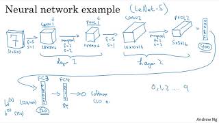
A short lecture walkthrough showing how to build a convolutional neural network for image recognition (example: 32x32x3 RGB input for digit recognition). The speaker gives a LeNet-5-inspired layer-by-layer architecture (conv and pooling layers followed by fully connected layers and a final softmax), explains shape/parameter calculations, and discusses conventions and hyperparameter choices.
Chapters
You now know pretty much all the building blocks of building a full convolutional neural network. Let's look at an example. Let's say that you're inputting an image which is 32 by 32 by 3. So it's an RGB image. And maybe you're trying to do handwritten digit recognition, you know, so you have a number like a 7 in a 32 by 32 RGB image, and you're trying to recognize which One of the ten digits from 0 to 9 this is. Let's build a neural network to do this. And what I'm going to use in this slide is inspired. It's actually quite similar to one of the classic neural networks called the Net5, which is created by Yann Lecun many years ago. What I'll show here isn't exactly the net 5, but is inspired by it. But many of the parameter choices was inspired by it. So with a 32 by 32 by 3 input, let's say that the first layer uses a 5x5 filter and a stride of one and no padding. So the output of this layer, if you use six filters, would be 28 by 28 by six. I'm going to call this layer conf1, right? So it applies six filters, add a bias, apply the non linearity, maybe a relu nonlinearity, and that's the conv1 output. Next, let's apply a pooling layer. So I'm going to apply max pooling here. And let's use f equals 2, s equals 2. When I don't write a padding, it means that padding is equal to 0. Next let's apply a pooling layer. I'm gonna apply, say max pooling with a two by two filter and a stride equals two. So this should reduce the height and width of the representation by a factor of two. So 28 by 28 now becomes 14 by 14 and the number of channels remains the same. So 14 by 14 by 6 and we're going to call this the Pool 1 output. So it turns out that in the literature of a convnet, there are two conventions which are slightly inconsistent about what you call a layer. One convention is that this is called one layer. So this would be layer one of the neural network. Another convention would be to count the conv layer as a layer and the pool layer as a layer. When people report the number of layers in a neural network, usually people report just the number of layers that have weights, that have parameters. And because the pooling layer has no weights, has no parameters, only a few hyperparameters. I'm going to use the convention that the conv1 and pool1 here together, I'm going to treat that as layer one. Although sometimes you see people, if you read articles online or read research papers, you hear about the conv layer and the pooling layer as if they are two separate layers. But this is maybe two slightly inconsistent notation terminologies. But when I count layers, I'm just gonna count layers that have weights. So I'm gonna treat both of these together as layer one. And the name conv1 and pool one I'm gonna use here. The one at the end also refers to the fact that I view both of these as part of layer one of the neural network. And pool one is grouped into layer one because it doesn't have its own weights. Now let's apply another convolutional layer to this. I'm going to use a five by five filter. So F equals five and a stride is one. And when I don't write the padding, it means there's no padding. And this will give you the conf2 output. And let's use 16 filters. So this would be a 10 by 10 by 16 dimensional output. So maybe look like that. And this is the conf2 layer. And then let's apply max pooling to this with f equals 2s equals 2. You can probably guess the output of this where 10 by 10 by 16 with max pooling with f equals 2s equals 2. This will halve the height and width. You can probably guess the result of this, right? Well, max pooling with f equals 2s equals 2. This should half the height and width. So you end up with a 5 by 5 by 16 volume, same number of channels as before. I'm going to call this pool two. And in our convention this is layer two, because you know, this has one set of weights in the conv two layer. Now, 5 by 5 by 16. 5 times 5 times 16 is equal to 400. So let's now flatten out pool two into a 400 by one dimensional vector, you know, so think of this as flattening this out into just a set of neurons, like so. And what we're going to do is then take this 400 units and let's build the next layer as having 120 units. So this is actually our first fully connected layer. I'm going to call this FC3 because we have 400 units densely connected to 120 units. So this fully connected unit. This fully connected layer is just like the single neural network layer that you saw in causes one and two. This is just a standard neural network where you have a weight matrix that's called W3 of Dimension 120 by 400. And this is called fully connected because each of the 400 units here is connected to each of the 120 units here. And you'd also have a bias parameter, I guess that's going to be just 120 dimensional because you have 120 outputs. And then lastly, let's take 120 units and add another layer, this time a little bit smaller. But let's say we have 84 units here. We're going to call this fully connected layer four. And finally you now have 84 row numbers that you can feed to a softmax unit. And if you're trying to do handwritten digit recognition, you have to recognize is it a handwritten 0, 1, 2 and so on up to 9, then this would be a softmax with 10 outputs. So this is a reasonably typical example of what a convolutional neural network might look like. And I know this seems like there are a lot of hyperparameters. We'll give you some more specific suggestions later for how to choose these types of hyperparameters. Maybe one guideline is to. One common guideline is to actually not try to invent your own settings of hyperparameters, but to look in the literature to see what hyperparameters you work for others and to just choose an architecture that has worked well for someone else. And there's a chance that will work for your application as well. We'll say more about that next week, but for now I just want to point out that as you go deeper in the neural network, usually NH and nw, the height and width will decrease. Pointed this out earlier, but it goes from 32 by 32 to 28 by 28 to 14 by 14 to 10 by 10 to 5 by 5. So. So as you go deeper, usually the height and width will decrease, whereas the number of channels will increase. It's gone from 3 to 6 to 16, and then you have fully convented layers at the end. And another pretty common pattern you see in neural networks is to have conv layers, maybe one or more conv layers followed by a pooling layer and then one or more conv layers followed by a pooling layer, uh, and then at the end to have a few fully connected layers and then followed by maybe a softmax. And this is another pretty common pattern you see in neural networks. So let's just go through, um, for this neural network, some more details of what are the activation shape, the activation size, and the number of parameters in this network. So the input was 32 by 30 by 3. And you multiply out those numbers, you should get 3072. So the activation, you know, a zero has dimension 3072. Well, it's really 32 by 32 by 3. And there are no parameters, I guess, in the input layer. And as you look at the different layers, feel free to work out the details yourself. These are the activation shape and the activation sizes of these different layers. So just on point of a few things, first, notice that the pooling layers, the max pooling layers, don't have any parameters. Um, second, notice that the conv layers tend to have relatively few parameters as, as we discussed in an earlier video. And in fact, a lot of the parameters tend to be in the fully connected layers of the neural network. And then you notice also that the activation size tends to maybe go down gradually as you go deeper into neural network. Um, if it drops too quickly, that's usually not great for performance as well. Right. So it starts in the first layer with 6,000, then, you know, 1,500, 1600, and then it kind of slowly falls into 84 until finally you have your softmax out plate and you find that a lot of convnets will have, you know, properties will have patterns similar to these. So you've now seen the basic building blocks of neural networks, of convolutional neural networks, the conv layer, the pooling layer, and the fully connected layer. A lot of computer vision research has gone into figuring out how to put together these basic building blocks to build effective neural networks. And putting these things together actually requires quite a bit of insight. Um, I think that one of the best ways for you to gain intuitions about how to put these things together is to see a number of concrete examples of how others have done it. So what I want to do next week is show you a few concrete examples, even beyond this first one that you just saw, on how people have successfully put these things together to build very effective neural networks. And through those videos next week, I hope they'll help you hone your own intuitions about how these things are built, um, as well as give you concrete examples of architectures that maybe you can just use, you know, exactly as developed by someone else for your own application. So we'll do that next week. But before wrapping up this week's videos, just one last thing, which is wanna talk a little bit in the next video about why you might want to use convolutions. Some of the benefits and advantages of using convolutions, as well as how to put it all together, how to take a neural network like the one you just saw and actually train it on a training set to perform image recognition or some of the tasks. So that. Let's go on to the last video of this.










