Three foundational CNN architectures: LeNet-5 for digit recognition, AlexNet which popularized ReLU and large-scale training, and VGG16 with its uniform 3x3 convolutions. The lecture walks through each network layer by layer, covering filter sizes, parameter counts, and why they mattered historically.
Chapters
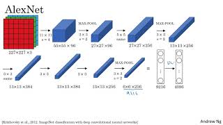
In this video, you learn about some of the classic neural network architectures, starting with Lenet 5 and then AlexNet and then vgg.net. let's take a look. Here's the Lenet 5 architecture. You start off with an image which say 32 by 32 by 1. And the goal of Lenet 5 was to recognize handwritten digits, so maybe an image of a digit like that. And the net 5 was trained on grayscale images, which is why it's 32 by 32 by 1. This neural network architecture is actually quite similar to the last example you saw last week. In the first step, you use a set of six 5 by 5 filters with a stride of 1. Because you use 6 filters, you end up with a 28 by 28 by 6 over there. And with a stride of 1 and no padding, the image dimensions reduces from 32 by 32 down to 28 by 28. Then the learnette neural network applies pooling. And back then when this paper was written, people used average pooling much more. If you're building a modern variant, you probably use max pooling instead. But in this example, you average pool, and with a filter width of two and a stride of two, you wind up reducing the dimensions, the height and width by a factor of two. So you now end up with a 14 by 14 by 6 volume. And I guess the height and width of these volumes aren't entirely drawn to scale. Technically, if I were drawing these volumes to scale, the height and width would be shrunk by a factor of two. Next you apply another convolutional layer. This time you use a set of 16 filters, they're five by five, so you end up with 16 channels in the next volume. And back when this paper was written in 1998, people didn't really use padding or you're always using valid convolutions, which is why every time you apply a convolutional layer, the height and width shrinks. So that's why here you go from 14 by 14 down to 10 by 10, then another pooling layer, so that reduces the height and width by a factor of two. And you end up with five by five over here. And if you multiply out these numbers five by five by 16, this multiplies out to 400, right? That's 25 times 16 is 400. And the next layer is then a fully connected layer that fully connects each of these 400 nodes with every one of 120 neurons. So there's a fully connected layer. And sometimes I would draw out, you know, explicitly a layer with 400 nodes. I'm skipping that here. There's a fully connected layer and then another fully connected layer. And then the final step is it uses these, you know, essentially 84 features and uses it with one final output. I guess you could draw one more node here to make a prediction for y hat. And y hat took on 10 possible values corresponding to recognizing each of the digits from 0 to 9. A modern version of this neural network would use a softmax layer with a 10 way classification output, although back then the Net5 actually used a different classifier at the output layer, one that's useless today. So this neural network was small by modern standards, had about 60,000 parameters. And today you often see neural networks with anywhere from 10 million to 100 million parameters. And it's not unusual to see networks that are literally about a thousand times bigger than this network. But one thing you do see is that as you go deeper in the NE network, so as you go from left to right, the height and width tend to go down. So you went from 32 by 32 to 28 to 14 to 10 to 5, whereas the number of channels tends to increase, it goes from 1 to 6 to 16 as you go deeper into the layers of the network. One other pattern you see in this neural network that's still often repeated today is that you might have some one or more conv layers followed by a pooling layer and then one or sometimes more than one conv layer followed by a pooling layer and then some fully connected layers and then the output. Right, so this type of arrangement of layers is quite common. Now finally, this is maybe only for those of you that want to try reading the paper. There are a couple other things that were different. The rest of this slide I'm going to make a few more advanced comments only for those of you that want to try to read this classic paper. And so everything I'm gonna write in red, you can safely skip on this slide. And this may be an interesting historical footnote that is okay if you don't follow fully. So it turns out that if you read the original paper back then, people used sigmoid and tanh nonlinearities, and people weren't using relu nonlinearities back then. So if you look at the paper, you see sigmoid and tanh referred to, and there are also some funny ways about this network was wired, at least funny by modern standards. So for example, you've seen how if you have a NH by NW by NC network with NC Channels, then you use F plus F by the same NC dimensional filter, where every filter looks at every one of these channels. But back then computers were much slower. And so to save on computation as well as on parameters, the original Learned five had some crazy complicated way where different filters look at different channels of the input block. And so the paper talks about those details, but the more modern implementation, you know, wouldn't have that type of complexity these days. And then one last thing that was done back then, I guess, but isn't really done right now, is that the original Learnet 5 had a nonlinearity after pooling. Right? And I think it actually uses sigmoid nonlinearity after the pooling layer. So if you do read this paper, and this is one of the harder ones to read of the ones we'll go over in the next few videos, um, the next one might be an easier one to start with. Most of the ideas on this slide are described in sections 2 and 3 of the paper. And later sections of the paper talk about some other ideas. Um, it talked about something called the graph transformer network, which isn't widely used today. So if you do try to read this paper, I recommend focusing on really on section two, which talks about this architecture, and maybe take a quick look at section three, which has a bunch of experimental results which are pretty interesting. The second example of a neural network I want to show you is Alexnet, named after Alex Trzhevsky, who was the first author of the paper describing this work. The other authors were Elias Suskever and Geoffrey Hinton. So AlexNet inputs starts with 227 by 227 x 3 images. Oh, and if you read the paper, the paper refers to 224 by 224 by three images. But if you look at the numbers, I think the numbers make sense only if it's actually 227 by 227. And then the first layer applies a set of 9611 by 11 filters with a stride of four. And because it uses a large stride of four, the dimension shrinks to 55 by 55, so roughly going down by a factor of four because of the last stride. And then applies max pooling with a 3x3 filter. So F equals 3 and a stride of 2. So this reduces the volume to 27 by 27 by 96. And then it performs a 5 by 5 same convolution. So with padding, so you end up with 27 by 27 by 276 max pooling. Again, this then reduces the height and width to 13. And then another same convolution. So same padding. So it's 13 by 13 by now, 384 filters. And then three by three, same convolution again gives you that. Then three by three, same convolution gives you that. Then MaxPool brings it down to six by six by 256. If you multiply out these numbers six times six times 256, that's 9216. So we're gonna unroll this into 9216 nodes. And then finally it has a few fully connected layers. And then finally it uses a softmax to output which 1 of 1000 classes the object could be. So this neural network actually had a lot of similarities to Learnet, but it was much bigger. So whereas Lenet or Lynette 5 from the previous slide had 60,000, about 60,000 parameters, this Alexnet had about 60 million parameters. And the fact that it could take, you know, pretty similar basic building blocks, but have a lot more hidden units and train it on a lot more data as they trained on the ImageNet dataset, that allowed it to have just remarkable performance. Another aspect of this architecture that made it much better than LUNET was using the RELU activation function. And then again, just if you read the paper, some more advanced details that you don't really need to worry about if you don't read the paper. One is that when this paper was written, GPUs were still a little bit slower. So it had a complicated way of training on two GPUs. And the basic idea was that a lot of these layers was actually split across two different GPUs. And there was a thoughtful way for when the two GPUs would communicate with each other and the paper also. The original Alexnet architecture also had another type of layer called a local response normalization. And this type of layer isn't really used much, which is why I didn't talk about it. But the basic idea of local response normalization is if you look at one of these blocks, one of these volumes that we have on top, let's say, for the sake of argument, this one, you know, 13 by 13 by 256, what local response normalization LRN does is it'll look at one position, so one position, height and width, and look down this across all the channels, look at all 256 numbers and normalize them. And the motivation for this local response normalization was that for each position in this 13 by 13 image, maybe you don't want too many neurons with a very high activation. But subsequently, many researchers have found that this doesn't help that much. So this, this is one of those ideas, I guess I'm drawing in red because it's less important for you to understand this one. And in practice, I don't really use local response normalizations, you know, really in, in the networks that I would train today. So if you're interested in the history of deep learning, I think even before Alexnet, deep learning was starting to gain TR and speech recognition and a few other areas. But, um, it was really this paper that convinced a lot of the computer vision community to take a serious look at deep learning, to convince them that deep learning really works in computer vision. And then it grew on to have a huge impact, uh, not just in computer vision, but beyond computer vision as well. And if you want to try reading some of these papers yourself, and you really don't have to for this course, but if you want to try reading some of these papers, this one is one of the easier ones to read. So this might be a good one to take a look at. So whereas Alexnet had a relatively complicated architecture, there's just a lot of hyperparameters, right, where you have all these numbers that Alex Kruzevsky and his co authors had to come up with. Let me show you a third and final example in this video called the VGG or the VGG16 network. And a remarkable thing about the VGG16 is that they said instead of having so many hyperparameters, let's use a much simpler network where you focus on just having conv layers that are just 3x3 filters with a stride of one, and always use the same padding and make all your max pooling layers two by two with a stride of two. And so one very nice thing about the VGG network was it really simplified these neural network architectures. So let's go through the architecture. So you start up with an image, and then the first two layers are convolutions, which are therefore these three by three filters. And in the first layers, first two layers, you use 64 filters. So you end up with a 224 by 224 because you're using same convolutions and, and then with 64 channels. So because VGG16 is a relatively deep network, I'm going to not draw all the volumes here. So what this little picture denotes is what we would previously have drawn as this 224 by 224 by 3 and then a Convolution that results in, I guess a 224 by 224 by 64. So be drawn as a deeper volume. And then another layer that results in, you know, 224 by 224 by 64. So this conf 64 times two represents that you're doing two layers, two conv layers with 64 filters. And as I mentioned earlier, the filters are always three by three with strider one and they're always same convolutions. So rather than drawing all these volumes, I'm just going to use text to represent this network. Next, then uses a pooling layer. So the pooling layer will reduce and think about it goes from 224 by 224 down to what? Right, goes to 112 by 112 by 64 and then it has a couple more conv layers. So this means it has a 128 filters. And because these are same convolutions. Let's see, what's the new dimension? Right, it'll be 112 by 112 by 128. Um, and then pooling layer, so you can figure out what's the new dimension. Right, it'll be that. And now three conv layers with two 56 dimensional filters. 256 filters, sorry. Then the pooling layer and then a few more conv layers, pooling layer, more conv layers, pooling layer. And then it takes this final 7 by 7 by 5 12, feeds it to fully connected layer, fully connected with 4096 units. And then the softmax output, one of a thousand classes. And by the way, the 16 in the name VG16 refers to the fact that this has 16 layers that have weights. And this is a pretty large network. This network has a total of about 138 million parameters. And that's pretty large even by modern standards. But the simplicity of the VGG16 architecture made it quite appealing. You can tell its architecture is really quite uniform. There's a few conv layers followed by a pooling layer, which reduces the height and width. So the pooling layers reduce the height and width. You have a few of them here, but then also if you look at the number of filters in the conv layers here, you have 64 filters and then you double to 128, double to 256, double to 512. And then I guess the authors thought five tail was big enough and didn't double again here. But this, you know, Sort of roughly doubling on every step or doubling through every stack of conv layers was another simple principle used to design the architecture of this network. And so I think the relative uniformity of this architecture made it quite attractive to researchers. The main downside was that it was a pretty large network in terms of the number of parameters you had to train. Oh, and if you read the literature, you sometimes see people talk about VGG19. That's an even bigger version of this network. And you can see the details in the paper cited at the bottom by Karen Simayan and Andrew Zisserman. But because VGG16 does almost as well as VGG19, a lot of people will use VGG16. But the thing I liked most about this was that this made this pattern of how, as you go deeper, height and width goes down, it just goes down by a factor of two each time for the pooling layers, whereas the number of channels increases. And here it, you know, roughly goes up by a factor of two every time you have a new set of conv layers. So by making the rate at which these go down and that go up very systematic, I thought this paper was very, very attractive from that perspective. So that's it for the three classic architectures. Uh, if you want, you should be able to now read some of these papers. I recommend starting with the Alexnet paper, followed by the VGG Net paper, and then the Lynette paper is a bit harder to read, but it is a good classic if you want to take a look at that. But next, let's go beyond these classic networks and look at some even more advanced, even more powerful neural network architectures. Let's go on to the next video.










