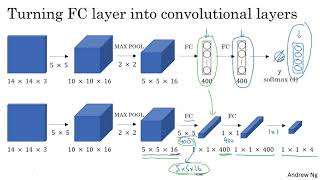
Converting fully connected layers to convolutional layers lets you run object detection on large images efficiently. Instead of sliding a window separately for each position, one forward pass produces outputs for all windows at once, sharing computation across the grid.
Questions this video answers
14×14×3 (training example); test examples include 16×16×3 and 28×28×3.
5×5 filters, 16 of them in the first conv layer; later using 5×5×16 filters to map to 400 outputs.
2×2 max pooling (effectively producing stride-2 downsampling).
400 units (represented as a 1×1×400 volume when converted to convolution).
Four classes (example: pedestrian, car, motorcycle, background).
Chapters
In the last video, you learned about the sliding Windows object detection algorithm using a continent, but we saw that it was too slow. In this video, you learn how to implement that algorithm convolutionally. Let's see what this means to build up toward the convolutional implementation of sliding Windows. Let's first see how you can turn fully connected layers in your neural network into convolutional layers. We'll do that first on this slide, and then the next slide. We'll use the ideas from this slide to show you the convolutional implementation. So let's say that your object detection algorithm inputs 14 by 14 by 3 images. This is quite small, but just for illustrative purposes. And let's say it then uses 5x5 filters and let's say uses 16 of them to map it from 14 by 14 by 3 to 10 by 10 by 16 and then does a 2x2 max pooling to reduce it to 5x5x16. Then has a fully connected layer to connect to 400 units, then another fully connected layer, and then finally outputs Y using a softmax unit. In order to make the change, we'll need to. In a second I'm going to change this picture a little bit and instead I'm going to view Y as four numbers corresponding to the class probabilities of the four classes that the softmax unit is classifying amongst. Um, and the four classes could be pedestrian, car, motorcycle, and background or something else. Now what I'd like to do is show how these layers can be turned into convolutional layers. So the convnet we're draw same as before for the first few layers. And now one way of implementing this next layer, this fully connected layer, is to implement this as a 5 by 5 filter. And let's use 405 by 5 filters. So if you take a 5 x 5 x 16 image and convolve it with a 5 by 5 filter. Remember, a 5 by 5 filter is implemented as 5 by 5 by 16, because our convention is that the filter looks across all 16 channels. So this 16 and this 16 must match. And so the output will be one by one. And if you have 400 of these 5 by 5 by 16 filters, then the output dimension is going to be one by one by 400. And so rather than viewing these 400 as just a set of nodes, we're going to view this as a 1x1x400 volume. And mathematically this is the same as a fully connected layer, because each of these 400 nodes has a filter of dimension 5 by 5 by 16. And so each of those 400 values is some arbitrary linear function of these 5 by 5 by 16 activations from the previous layer. Next, to implement the next convolutional layer, we're going to implement a one by one convolution. And if you have 400 one by one filters, then with 400 filters, the next layer will again be one by one by 400. So that gives you this next fully connected layer. And then finally we're going to have another one by one filter followed by a softmax activation so as to give a one by one by four volume to take the place of these four numbers that the network was outputting. So this shows how you can take these fully connected layers and implement them using convolutional layers so that these sets of units instead are now implemented as one by one by 401, one by one by four volumes. Armed with this conversion, let's see how you can have a convolutional implementation of Sliding Windows object detection and the presentation on this slide is based on the Overfeed paper referenced at the bottom by Pierre Cerbni, David Eigen, Xiang Zhang, Michael Matthew, Rob Fergus and Yann Lecun. Let's say that your Sliding Windows ConvNet inputs 14 by 14 by 3 images. And again, I'm just using small numbers like a 14 by 14 image in this slide, mainly to make the numbers and illustrations simpler. So as before, you have a neural network as follows, that eventually outputs a one by one by four volume, which is the output of your softmax unit. And again, to simplify the drawing here, 14 by 14 by 3 is technically a volume 5 by 5 or 10 by 10 by 16, it's technically a volume. But to simplify the drawing for this slide, I'm just going to draw the front face of these volumes. So instead of drawing, you know, one by one by 400 volume, I'm just going to draw the one by one parts of all of these, right? So just drop the 3D component of these drawings just for this slide. So let's say that your convnet inputs 14 by 14 images or 14 by 14 by 3 images. And your test set image is 16 by 16 by 3. So I've now added that yellow stripe to the border of this image. So in the original Sliding Windows algorithm, you might want to input the blue region into a convnet and run that once to generate a classification 01 and then slide it down a bit let's use a stride of two pixels and and then you might slide and then you might slide that to the right by 2 pixels to input this green rectangle into the convnet and rerun the whole convnet and get another label 01. And then you might input this orange region into the convnet and run it one more time to get another label and then do it the fourth and final time with this, your lower right now purple square. And so to run sliding windows on this 16 by 16 by 3 image is pretty small image. You run this convnet from above four times in order to get four labels. But it turns out a lot of this computation done by these four convnets is highly duplicated. So what a convolutional implementation of sliding windows does is it allows these four forward passes of the confnet to share a lot of computation. Specifically, here's what you can do. You can take the confnet and just run it, same parameters, the same 5 by 5 by filters, all 165 by 5 filters and run it. And now you can have a 12 by 12 by 16 output volume and then do the max pull same as before. Now you have a 6 by 6 by 16 runs through your same 405 x 5 filters to get now your 2 by 2 by 40 volume. So now instead of a 1 by 1, so now instead of a 1 by 1 by 400 volume, you have instead a 2 by 2 by 400 volume. Run it through a 1 by 1 filter gives you another 2 by 2 by 400 instead of 1 by 1 by 400. Do that one more time and now you're left with a 2 x 2 x 4 output volume instead of 1 x 1 x 4. And it turns out that this blue 1 by 1 by 4 subset gives you the result of running in the upper left hand corner 14 by 14 image. This upper right 1x1x4 volume gives you the upper right result. The lower left gives you the results of implementing the confnet on the lower left 14 by 14 region. And the lower right one by one by four volume gives you the same result as running the confnet on the lower right 14 by 14 region. And if you step through all the steps of the calculation. Let's look at a green example. If you had cropped out just this region and passed it through the confnet through the confnet on top, then the first layer's activations would have been exactly this region. The next layer's activation after max pooling would have been exactly this region and then the next layer, the next layer would have been as follows. So what this process does, what this convolutional implementation does is instead of forcing you to run forward propagation on four subsets of the input image independently, instead it combines all four into one forward prob computation and shares a lot of the computation in in the regions of the image that are common to all four of the 14 by 14 patches we saw here. Now, let's just go through a bigger example. Let's say you now want to run sliding windows on a 28 by 28 by 3 image. It turns out if you run forward Prof. The same way, then you end up with an 8x8x4 output. And this corresponds to running sliding windows with that 14 by 14 region. And that corresponds to running sliding windows first on that region, thus giving you the output corresponding to the output left hand corner, then using Strider 2 to shift one window over, one window over, one window over,' and so on. And they're eight positions. So that gives you this first row and then as you go down the image as well, that gives you all of these 8 by 8 by 4 outputs and BE. And it's because of the max pooling of two that this corresponds to running your neural network with a stride of two on the original image. So just to recap, to implement sliding windows previously, what you do is you crop out a region, let's say this is 14 by 14, and run that through a confnet, and do that for the next region over, then do that for the next 14 by 14 region, then the next one, then the next one, then THE next one, then THE next one, and so on, until hopefully that one recognizes the car. But now, instead of doing it sequentially, with this convolutional implementation that you saw on the previous slide, you can implement the entire image, all maybe 28 by 28, and convolutionally make all the predictions at the same time. By one thought it passed through this big continent and hopefully have it recognize the position of the car. So that's how you implement sliding windows convolutionally, and it makes the whole thing much more efficient. Now, this algorithm still has one weakness, which is the position of the bounding boxes is not going to be too accurate in the next video. Let's see how you can fix that problem.