C4W4L11 1D and 3D Generalizations
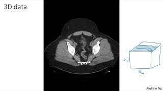
Andrew Ng explains how convolutional networks extend from 2D images to 1D time-series like EKG signals and 3D volumetric data like CT scans or videos. The same filter logic applies across dimensions: a 5×5×3 filter on a 14×14×3 image produces a 10×10×16 output, just as a 5×5×5 filter works on 14×14×14 volumes.
Chapters
You've learned a lot about convnets. Everything ranging from the architecture of a convnet to how to use it for image recognition, to object detection, to face recognition and neural style transfer. And even though most of our discussion has focused on images on sort of 2D data, because images are so pervasive, it turns out that many of the ideas you've learned about also apply not just to 2D images, but also to 1D data as well as to 3D data. Let's take a look. In the first week of this course, you learned about the 2D convolution, where you might input a 14 by 14 image and convolve that with a 5x5 filter. And you saw how 14 by 14 convolved with 5x5, this gives you a 10 by 10 output. And if you had multiple channels, maybe those 14 by 14 by 3, then it would be 5 by 5 that matches the same three. And then if you have multiple filters, say 16 filters, you end up with 10x10x16. It turns out that a similar idea can be applied to 1D data as well. For example, on the left is an EKG signal, also called an electrocardiogram. Basically, if you place an electrode over your chest, this measures the little voltages that vary across your chest as your heart beats, because the little electric waves generated by your heart beating can be measured with a pair of electrodes. And so this is an EKG of someone's heart beating. And so each of these peaks corresponds to one heartbeat. So if you want to use EKG signals to make medical diagnoses, for example, then you would have 1D data, because what EKG data as is is basically a time series showing the voltage at each instant in time. So rather than a 14 by 14 dimensional input, maybe you just have a 14 dimensional input. And in that case, you might want to convolve this with a 1:1 dimensional filter. So rather than the 5x5, you just have a 5 dimensional filter. So with 2D data, what the convolution allow you to do is to take the same five by five feature detector and apply it at lots of different positions throughout the image. And that's how you wound up with your 10 by 10 output. What a 1D filter allows you to do is take your five dimensional filter and similarly apply that at lots of different positions throughout this 1D signal. And so if you apply this convolution, what you find is that a 14 dimensional thing convolved with this five dimensional thing, this would give you a 10 dimensional output. And again, if you have multiple channels, you might have a 14 by in this case an EKG is just one channel. If you have one lead or one electrode for your EKG. So times 5 by 1 and if you have 16 filters, maybe you end up with 10 by 16 over there. And this could be one layer of your convnet. And then for the next layer of your convnet, if you input a 10 by 16 dimensional input and you might convolve that with a 5 dimensional filter, again then this needs to have 16 channels, so that has to match. And if you have three 32 filters, then the output after another layer would be 6 by 32. If you have 32 filters, right. And the analogy to the 2D data is this is similar to how if you have 10 by 10 by 16 data and you convolve it with a 5 by 5 by 16 and that has to match, that will give you a 6 by 6 dimensional output. And if you have 32 filters, that's where the 32 comes from. So all of these ideas apply also to 1D data, where you can have the same feature detector such as this applied to a variety of positions, for example, to detect the different heartbeats in an EKG signal, but to use the same set of features to detect the heartbeats even at different positions along these time series. And so confidence can be used even on 1D data. For a lot of 1D data applications, you actually use a recurrent neural network which you learn about in the next course. But some people also can try using confidence in these problems. And in the next course on sequence models, which we'll talk about recurrent neural networks and LCM and other models like that, we'll talk about the pros and cons of using 1D confnets versus some of those other models that are explicitly designed for sequence data. So that's the generalization from 2D to 1D. How, how about 3D data? Well, what is three dimensional data? It is that instead of having a 1D list of numbers or a 2D matrix of numbers, you now have a 3D block, a three dimensional input volume of numbers. So here's an example of that, which is if you take a CT scan, this is a type of X ray scan that gives a three dimensional model of your body. But what a CT scan does is, is it takes different slices through your body. So as you scan through a CT scan, which I'm doing here, you can look at different slices of the human torso to see how they look, and so this data is fundamentally three dimensional. And one way to think of this data is if your data now has some height, some width and then also some depth, where this is where the different slices through this volume are the different slices through the torso. So if you want to apply a convnet to detect features in this three dimensional CAT scan or CT scan, then you can generalize the ideas from the first slide to three dimensional convolutions as well. So if you have a 3D volume, and for the sake of simplicity, let's say is 14 by 14 by 14. And so this is the height, width and depth of the input CT scan. And again, just like images don't all have to be Square, a 3D volume doesn't have to be a perfect cube as well. So the height and width of an image can be different. And in the same way the height and width and the depth of a CT scan can be different. But I'm just using 14 by 14 by 14 here to simplify the discussion. And if you convolve this with a now a 5 by 5 by 5 filter, so your filters now are also three dimensional, then this will give you a 10 by 10 by 10 volume. And technically you could also have by one. If this is the number of channels, so this is just a 3D volume, but your data can also have different numbers of channels, then this would be times one as well, because the number of channels here and the number of channels here has to match then. And if you have 16 filters that are 5 by 5 by 5 by 1, then the next outputs will be 10 by 10 by 10 by 16 and then if so this could be one layer of your confnet over 3D data. And if the next layer of the confnet convolves this again with a 5 by 5 by 5 by 16 dimensional filter, so this number of channels has to match that as usual. And if you have 32 filters, then similar to what you saw with confnet over images now you end up with a 6 by 6 by 6 volume across 32 channels. So 3D data can also be learned on sort of directly using a three dimensional conflict. And what these three filters do is really detect features across your 3D data. Cat scans, medical scans is one example of 3D volumes. But another example of data you could treat as a 3D volume would be movie data where the different slices could be different slices in time through a movie. And you could use this to detect motion or people taking actions in movies. So that's it on generalization of confidence from 2D data to also 1D, as well as for 3D data. Image data is so pervasive that the vast majority of convnets are on 2D data on image data, but I hope that these other models will be helpful to you as well. So this is it. This is the last video of this week and the last video of this course on convnets. You've learned a lot about convnets, and I hope you find many of these ideas useful for your future work. So congratulations on finishing these videos. I hope you enjoyed this week's prone exercise, and I look forward also to seeing you in the next course on sequence models.










