Dropout Regularization (C2W1L06)
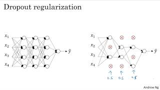
Andrew Ng explains dropout, a regularization technique that randomly zeros hidden units during training with a keepprob parameter (like 0.5 or 0.8). Inverted dropout divides activations by keepprob to maintain expected magnitude, eliminating the need to scale at test time when the full network runs.
Questions this video answers
0.5 and 0.8.
After applying the dropout mask, divide the masked activations by keepprob (e.g., a3 /= keepprob) so expected activation magnitude remains unchanged.
No; at test time the full network is used without applying dropout masks.
Chapters
In addition to L2 regularization, another very powerful regularization technique is called dropout. Let's see how that works. Let's say you've trained a neural network like the one on the left and is overfitting. Here's what you do with dropout. Let me make a copy of the neural network with dropout. What we're going to do is go through each of the layers of the network and set some probability of eliminating a node in a neural network. So let's say that for each of these layers, we're going to, for each node, toss a coin and have a 0.5 chance of keeping each node and 0.5 chance of removing each node. So after the coin tosses, maybe we'll decide to eliminate those nodes. Then what you do is actually remove all the ingoing outgoing links from that node as well. So you end up with a much smaller, really much diminished network. And, and then you do backpropagation, training this one example on this much diminished network. And then on different example, you would toss a set of coins again and keep a different set of nodes, drop out or eliminate a different set of nodes. And so for each training example, you would train it using one of these, you know, reduced networks. So maybe this seems like a slightly crazy technique to just go, go around culling nodes at random, but this actually works. But you can imagine that because you're training a much smaller network on each example, maybe, you know, this gives a sense for why you end up able to regularize the network, because these much smaller networks are being trained. So let's look at how you implement dropout. There are a few ways of implementing dropout. I'm gonna show you the most common one, which is a technique called inverted dropout. Um, for the sake of concreteness, let's say we illustrate this with layer L equals 3. So in the code I'm going to write, there'll be a bunch of threes here. That's just, you know, that I'm just going to illustrate how to implement dropout in a single layer. So what we're going to do is set a Vector D and D3 is going to be the dropout vector for layer 3. That's what the 3 is to be. NP, random, rand. And this is going to be the same shape as a three. And I'm going to see if this is less than some number, which I'm going to call keepprob. And so Keepprob is a number. It was 0.5 on the previous slide, but maybe now I'll use 0.8 in this example and it'll be the probability that a given hidden unit will be kept. So if keyprop is equal to 0.8, then this means that there's a 0.2 chance of eliminating any hidden unit. So what this does is it generates a random matrix. And this works as well if you have vectorized. So D3 will be a matrix where for each example and for each hidden Unit, there's a 0.8 chance that the corresponding D3 will be 1 and a 20% chance there'll be 0. Right? So you know this, this random number being less than 0.8, that has a 0.8 chance of being 1 or being true and a 20% chance of 0.2 chance of being false of being 0. And then what you're gonna do is take your activations from the third layer. Let's call that a3 in this little example. So a3 are the activations you computed, and you're gonna set a3 to be equal to the old a3 times. Okay, so this is an element wise multiplication, or I guess you could also write this as a three times equals D3. But what this does is for every element of D3 that's equal to zero, and there was a 20% chance of each of the elements being zero, you end up, this multiply operation ends up zeroing out the corresponding element of D3. If you do this in Python, technically D3 will be a boolean array with values true and false rather than 1 and 0. But you know, multiply, the multiply operation works and it'll interpret the true and false values as 1 and 0. If you try this yourself in Python, you, you see, then finally we're going to take a 3 and scale it up by dividing by 0.8 or really dividing by our heap prop parameter. So let me explain what this final step is doing. Let's say for the sake of argument that you have 50 units or 50 neurons in the third hidden layer. So maybe a three is 50 by one dimensional, or if you factorization, maybe it's 50 by M dimensional. So if you have a 80% chance of keeping them, 20% chance of eliminating them, this means that on average you end up with 10 units, you know, shut off or 10 units zeroed out. And so now if you look at the value of z4, z4 is going to be equal to w4 times a3 plus b4 and so on expectation, this will be reduced by 20%, by which I mean that 20% of the elements of a3 will be zeroed out. So in order to not reduce the expected value of Z4, what you do is you need to take this and divide it by 0.8, because this will, you know, correct, or this will bump it back up by the roughly 20% that you need so as to not change the expected value of a 3. And so this line here is what's called the inverted dropout technique. And its effect is that no matter what you set the keyprop to, whether it's 0.8 or 0.9 or even 1, if you set to 1, then there's no dropout because you're keeping everything, or 0.5 or whatever. This inverted dropout technique, by dividing by the key prop, it ensures that the expected value of a 3 remains the same. And it turns out that at test time, when you're trying to evaluate the neural network, which talk about in the next slide, this inverted dropout technique, there's this line test that drew the green box around. This makes test time easier because you have less of a scaling problem. But by far the most common implementation of dropout today, as far as I know, is inverted dropout. So I recommend you just implement this. But there were some early iterations of dropout that missed this divide by keyprob line. And so at test time, the algorithm became a little bit more complicated. But. But again, people tend not to use those other versions. So what you do is you use the D vector and you notice that for different training examples, you zero out different hidden units. And in fact, if you make multiple passes through the same training set, then on different passes through the training set, you should randomly zero different hidden units. So it's not that, for one example, you should keep zeroing out the same hidden units is that on iteration one of gradient descent, you might zero out some hidden units. And on the second iteration of gradient descent, where you go through the training set a second time, maybe you zero out a different pattern of hidden units. And the Vector D or D3 for the third layer is used to decide what to zero out, both in forward prop as well as in back prop. We're just showing forward prop here. Now, having trained the algorithm at test time, here's what you would do. At test time, you're given some X on which you want to make a prediction. And using our standard notation, I'm gonna use a 0, the activations of the 0th layer to denote this test example X. So what we're going to do is not use dropout at test time. In particular, we're just gonna set z1 equals w1 a0 plus b1 a1 equals g1 of z1, z2 equals w2 a1 plus b2 a2 equals. And so on until you get to the last layer and then you make a prediction Y hat. But notice that at test time, you're not using Dropout explicitly in that you're not tossing coins at random, you're not not flipping coins to decide which hidden units to eliminate. Um, and that's because when you're making predictions at test time, you don't really want your output to be random. If you were implementing Dropout at test time, that just add noise to your predictions. In theory, one thing you could do is run a prediction process many times with different hidden units randomly dropped out and then average across them. But that's computationally inefficient and it gives you roughly the same result. Very, very similar result to this particular procedure as well. And I just mentioned the inverted dropout thing. Remember the step on the previous slide where we divided by the keep prop? The effect of that was to ensure that even when you don't implement Dropout at test time to the scaling, the expected value of these activations don't change. So you don't need to add in an extra funny scaling parameter at test time that's different than what you had at training time. So that's dropout. And when you implement this in this week's program exercise, you gain more first hand experience with it as well. But why does it really work? What I want to do in the next video is give you some better intuition about what Dropout really is doing. Let's go on to the next video.










