Learn How to Build Multimodal Search and RAG

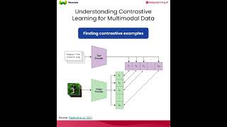
In this lesson, you'll learn about multimodality, what multimodal models are, and more specifically, how to teach a computer the concept of understanding multimodal data through the process of contrastive representation. Learning. Alright, let's dive in to stir your imagination. Let's start with a live multimodal search demo to see how you can search across different types of content. Here you can see that I can provide a text input, so I can search for a bunch of lions, and and I can get back images, audio and video files. And in this course we'll go over how this actually works. I'll explain the technology that powers this app, and you'll learn hands on how to build similar functionality. We won't necessarily build this app, but by the end of this course, you should know enough to build apps like this one and more. So why should you learn about multimodality? Multimedia content is all around us. Whether we are searching through our favorite songs, looking for movies to watch, browsing for things to buy, or looking for a Wikipedia article, everything that we do starts with search. But we don't want to just search through text. We want to search through songs, movie trailers, product images. We want to search through multimodal data. But what is multimodal data anyway? Multimodal data is data that comes from different sources. It can include text, images, audio and video, and much more. And each of those modalities often describe similar concepts. We could have a picture of a lion, a paragraph describing the king of the jungle, a video of running lions, or even the sound of a lion roar. Each modality comes with a different kind of information, and by combining the information, we gain better understanding of the concepts they represent. Think of it. It is more impressive or even scary to see and hear a lion roar than just watching quietly. After all, it is only when you see the lion and hear him, you understand why he is the king of the jungle. Another motivation behind why we want to learn from multimodal data is to think about how humans learn. Think of a child in their first year of life, before they learn to speak. A lot of their learning is done to interactions with objects. They touch, smell, feel the texture of, or even taste, even if it's soap, but also by watching and listening to everything around them. So this foundational knowledge is built using multimodal interactions with the world, and not by using a language. Now, if you want to build a smarter and more capable AI, it also needs to learn and think about different modalities of information, just like humans do to get computers to work with multimodal data, we need to first learn about multimodal embeddings. Multimodal embeddings allow us to represent multimodal data on the same vector space so that a picture of a lion will be placed close to a text describing lions, and also a lion roar or a video of running lions will be there. And we can generate these embeddings from many different sources. Multimodal embedding models produce a joint embedding space that understands all of your modalities. You can understand emails, you can understand images, audio files, and much more. The key concept here is that this model preserves semantic similarity within and across modalities. That means if you have objects that are similar regardless of the modality, their vectors will be close together like a picture of a lion and a related description, while different concepts like lions and trumpets are far from each other in the multimodal space. In order to start training multimodal embedding models, you need to start with a model that understands one modality at a time. These individual models are specialized at understanding text. Another separate model might capture representation of images and other models specializing in audio and video. The next task is to unify these models so that regardless of modality, similar concepts should result in closed vectors. So, on the left hand side, all of these concepts are similar and therefore the vectors that they generate on the right hand side should are also similar to each other. The task of unifying multiple models into one embedding space is done using a process called contrastive representation learning. Contrastive representation learning is a general purpose process that can be used to train any embedding model, not just multimodal embedding models. Specifically here, though, it can also be used to unify multiple models into one multimodal embedding model. With the main idea where we want to create one unified vector space representation for multiple modalities, we do it by providing our models with positive and negative examples of similar and different concepts. Then we train our models to pull closer vectors for similar examples and push further vectors for different concepts. So let's work through a text example to understand how this works. First we need an anchor point. This can be any data point. For example, he could smell the roses. Then we need a positive example, an example that is similar to the anchor, like a field of fragrant flowers. And finally we need a negative example, one that is dissimilar to the anchor, like the lion roared majestically. Now we can get the vector embedding for each data point, and we want to Push away the negative vector from the anchor and pull the positive vector closer to the anchor. We could use the same method to train an image model where the anchor could be a picture of a German shepherd, the positive example could be a grayscale version of the anchor, while the negative example could be a picture of an owl. And again, the task is to push away the negative example and pull closer the positive example. The pushing and pulling process is achieved with the contrastive loss function. First, we need to encode the anchor and the examples into vector embeddings. Then we calculate the distance between the anchor and the examples. And during the training process, we want to minimize the distance between the n curve vector and positive example vectors, while at the same time maximizing the distance to the negative example vectors. Now let's expand the concept of contrastive learning to multimodal data. We can provide positive and negative examples in different modalities. So, given our anchor is a video of Ryan lions, we can provide contrastive examples as images and text. Then we can apply pushing and pulling across modalities, and as a result, align the model to work in the same vector space across all modalities. One tricky part can be finding enough of anchors and contrastive examples. In a clip paper from 2021, they took images as their corresponding captions, each representing a different modality. The picture in its caption represented an anchor and a positive example as represented on the diagonal of this matrix. While any other random pairing of a picture and a caption is likely to be a negative example. And with that, they were able to apply contrastive loss function to train the text and image multimodal model. Now let's see how a contrastive function looks like. First, you need encoding functions that can convert the anchor and contrastive examples into vectors of the same dimension. Here we've got a function S that takes an image and returns a vector Q. And here we've got a function G which takes a video and generates vector K. Now you take those vector representations and the numerator, you've got a similarity between positive examples. So this could be the image of a lion and a video of running lions. You want the similarity to be as high as possible in the denominator. Here you've got a negative example, say.

The image of a lion and a.

Couple of kittens on a bicycle. This, in fact, is one of many negative examples that you need to sum up. You want this formula to return a probability. So in the denominator you normalize by providing the positive example from the numerator again and up front, you have a negative on this loss function, which means that you actually want to minimize it. And by minimizing this, the positive video embeddings will be pulled closer to the anchor image embedding and and the negative video will be pushed away from the anchor image. You can do this for all the modalities, one by one, for audio, for text, for video, and many more. And this is what they did in the image bind paper. Let's now see all of this in practice. In the lab, you train an embedding model using contrastive loss, then visualize the learned vector space.

All right, let's code. In this lab, you train a neural network to learn embeddings for the mnist image dataset. But let's start by running this code, which will simply ignore any warnings that are not necessarily important for us to analyze. So, first thing you are going to do is import the required libraries. You're going to use Pytorch for training the model and a set of supporting libraries. And the most important ones are libraries for visualization like Plotly and umap.

And the last thing that you need.

To import is the mnist dataset class, which you use to get positive and negative examples to train and Test on. The MNIST dataset is based on images of digits from 0 to 9. And each image of a digit is labeled with the value that it corresponds to, so that we know whether it represents 0 or a 5 or a 9. And the dataset class provides you with an anchor, which is a digit, and a positive and negative example, which are also digit examples, just like we talk about in the slides. For example, if the anchor is a 5, then a positive example would be another image for a 5, while a negative example would be an image of, let's say, six or a seven. And if you're curious about the mnist dataset code, feel free to review the mnistataset PY file. And in here there are two key parts that you should pay attention to. This bit of code over here takes care of labeling positive and negative examples so that when the label from the anchor matches the eye, that automatically means that this is a positive example. This is when you have a 7 and a 7, while if these values differ, so maybe the anchor is 7 while the example is 5, then this is assigned to the negative labels list. And the second key part is the code over here, which takes care of allocating the ideal distance metric that you will use during training. And since you use cosine similarity, the ideal Similarity between positive examples and anchor is set to 1, while for negative examples this is set to 0. And in a nutshell, these are the two key parts that allow you to find the positive and negative examples and allocate ideal distances to each example. All right, let's get back to the training notebook. So now let's load the data from the MDIST dataset. And here are the training dataset and the validation dataset that you need to load. And then let's execute this and this will load the dataset for you. Okay, great. And once the dataset is loaded, you need to set up Pytorch data loaders that will feed the neural network to train on. So feel free to modify this batch size over here if you want to see how that changes the convergence of the training. So, yeah, let's run this. Now let's use the above data loaders to visualize the anchor points and the corresponding positive and negative examples. First, add a helper function that will display provided images. And then you need to loop through the batch of the datasets from the trained data loader. And from here, what you'll be grabbing is the anchor images, the contrasted images, their ideal distances and their labels. And if you run this, you should get examples of like four images of each. And here you can see one anchor, which is a nine, and a positive example which is another nine. There is an eight and a six. So this is a negative example, another positive example, and a 4 and a 7, which should be used as a negative example. And that's basically what we will use for pushing and pulling to train this neural network. All right, you're doing great. Now let's define a neural network architecture that will take the MNIST images and output them as 64 dimensional vectors. So this is a simple architecture. We have two convolutional layers, and the point of these convolutional layers is to extract the visual features of a digit. Then you have two feedforward linear layers here, and their job is to make visual features learned by the convolution layer and learn how to turn them into 64 dimensional representations. And all of this is combined in this forward function. So in summary, you pass an image at the top, then you run through the two convolutional layers, flatten the output from that, and and then finally pass it through a linear function. And at the end you get a 64 dimensional vector. And that's basically how your neural network architecture looks like. Now, to train the neural network, you use the contrastive Loss function, which will take the 64 dimensional vector representations for both the anchor and then either a positive or negative example. And then you will make sure that the ideal distances are met. So like discussed earlier, the ideal cosine distance for a positive sample is 1 and a negative is 0.

This is probably the most important part.

Of this codalong, so let's dive into it. So here you define the contrastive loss as calculating a cosine similarity between two points. In the forward function you have the anchor and a contrastive example which could be either a positive or a negative one, together with their ideal distance. So the forward function is implemented as a two step thing. So first we calculate the score cosine similarity between the anchor and the contrastive images. And in the second step this score is compared to the ideal distance that you expect. And here's a key information, lower distance between these two scores mean lower loss, and you want to eventually minimize this loss. So by the time this neural network is trained, the calculated score should be very close to the expected ideal distance. And here you use CPU for training as the default option. However, if the GPU or CUDA are available, then in this case that would be used instead of the cpu. And you also need to add in the configuration parameters for the neural network training. So this is your optimizer, this is actually what does the gradient descent. Then you need to set up contrastive loss function. And here is your training scheduler. And now you are getting to the fun part, the code that executes the training of this model. So first to help us set it all up, we need a checkpoints folder where the results of the training will be saved into that you could actually use later on to reload all the training back. And now let's have a look at the training loop. You can set it to run over any number of epochs. And the training loop goes through and trains the model, which goes through forward propagation and backwards propagation until it converges. And one of the key parts to see in here is the loss function, which takes the anchor and the contrastive vectors together with their expected distances and calculates the loss for each data point. The loss is then added up, which at the end of the epoch is used to calculate the average loss for each epoch, which is how you know whether the model training is improving or not. And also, as each epoch is completed, the loop saves the results into the checkpoint folder. And finally, what the function returns back is the train model together with an array of the losses epoch by epoch. And this is in a Nutshell, how the training works. Please note though that the training process is rather slow, so it can take two to three minutes per epoch. So it can take quite a while to run across 10, 20 or even 100 of them. But don't worry, we have a backup plan and we already pre trained this model over 100 epochs. And in the interest of time, I suggest loading the pre trained model from the provided checkpoint instead of training the model from scratch. Now run the following code to get your model and by default this will try and load the model from the checkpoint. However, if you'd like to run the full training yourself, you can change this train flag to true. Remember, this is a lengthy process, so you need to be very patient when you do run this and let's run this and you should straight away get the ready model. If you did choose to train the model yourself, then you can plot out how the loss was changing over the epochs. And you can see that in our case the training was pretty much settled around the 20 epochs. So most of the learning was done in the first five to 10 and then around 20 were already settled and then there was only minute changes and improvements over time. Great, so this part's done. And now that you have a trained neural network, you can visualize the vector space and see what was actually learned. To visualize the vector space you need to take the training data set and then encode it all with the model. And as a result you get 64 dimensional vector representation of the data. You also need the labels for each item so that you could display each digit in a different color. Now let's run it to get our encoded data together with the labels. And this shouldn't take too long, so just bear with it. And because we don't see the world in 64 dimensions, you need to do another further dimensionality reduction step. So here you're going to use a concept called principal component analysis. And, and this will take you from 64 dimensions to 3 dimensions which we should be able to see. And now that you have the 3D vectors, you can actually visualize this data in an interactive scatter plot. So here take the three dimensional data that you reduced in the previous step across X, Y and z axis and then use it to create a plotly graph object layout which we then can call to show and then display it like this. And when you plot this out, you see the vectors plotted on this graph where each color represents a different point for a different digit. So in here we have sevens, we have threes, and twos and sixes, etc. And because you use cosine distance metric for the training, the embeddings for similar digits align in a spoke or let's say line shape rather than a cluster, like this six digits here. And this is because cosine distances depend on angles between embeddings, unlike Euclidean distance, which minimizes proximity. And you can move around this. So if you hold the left mouse button, you can see the space from different angles. With the right mouse you can move left and right and then you can also scroll in to zoom in a bit closer. What we see on the graph, One note though, because we compress the vectors from 64 dimensions to 3 dimensions, it still may look like maybe some of the embeddings are kind of like still very close to each other, like this two and four. It kind of depends on which angle you are looking at at this. But also reducing it from 64 dimensions to 3 dimensions can do it like that. But the overall thing is that like for most of the digits, you can very visibly see how each of them is pointing in a different direction, as you would expect from a cosine based training. And next you can use this technique called UMAP to visualize the train embeddings on a 2D space. Notice that the metric provided here is set to cosine. And this is really important to note because UMAP defaults to Euclidean distance, which wouldn't give you an accurate view of the vector embedding space. So let's run this. And please note, this can take half a minute, up to a minute to complete. So be patient. And eventually the 2D plot will show and in this chart each digit is represented by a different color, just like before. And you can see how digits are clustered in a jellyfish like pattern. I guess this is where deep learning crosses over with deep C. You never know. But overall this demonstrates that the contrastive training was successful. And each digit's representation is clustered in a separate part of this vector space. And out of curiosity, if you run the same code without specifying the distance metric, UMAP will use Euclidean distance. And you get a bunch of strings like this one, and you can still see that those strings are close together and they like sort of follow each other. And who knows, maybe this is the answer to the string theory. I'm just kidding. Don't call Sheldon Cooper. And finally you have this video that you can play yourself to see the training process of the contrasting learning over 100 epochs.

And you can see how at the.

Beginning, the data points are all clustered together, but over time, similar embeddings get aligned while different numbers spread out in other directions. And this is the effect of pulling similar examples closer together and pushing different examples further apart. And in a nutshell, that's how contrastive training works. In this lesson, you've learned how to implement contrastive learning to train a neural network on an image dataset.

You learned also how pushing and pulling.

Of negative and positive examples help help train the model. And finally, you use PCA and UMAP to plot reduced emotionality vector embeddings to analyze results of the training of a vector space. In the next lesson, you'll learn how to use a vector database with a multimodal model to vectorize images and videos, and then search with text image and video input.

Great.

I'll see you.