Instructor explains why the common low-dimensional intuition of many bad local optima is misleading for neural network training. In high-dimensional parameter spaces, most stationary points (zero gradient) are saddle points rather than local minima; plateaus—regions with near-zero gradient—can severely slow learning. Optimizers such as Momentum, RMSProp, and Adam can help escape plateaus and accelerate convergence. The video is part of a course module (mentions weekly quiz and pro exercise).
Chapters
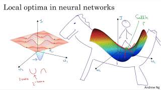
In the early days of deep learning, people used to worry a lot about the optimization algorithm getting stuck in bad local optima. But as the theory of deep learning has advanced, our understanding of local optima is also changing. Let me show you how we now think about local optima and problems with the optimization problem in deep learning. So this was a picture people used to have in mind when they worried about local optima. Maybe you're trying to optimize some set of parameters, I'm going to call them W1 and W2, and the height of the surface is the cost function. So in this picture it looks like there are a lot of local optima, you know, in, in all those places. And it'd be easy for gradient descent or one of the other algorithms to get stuck on a local optimum rather than find its way to a global optimum. It turns out that if you're plotting a figure like this in two dimensions, then it's easy to create plots like this with a lot of different local optima and these very low dimensional plots used to guide our intuition. But this intuition isn't actually correct. It turns out if you train a neural network, most points of zero gradients are not local optimal, like points like this. Instead, most points of zero gradient in a cost function are actually saddle points. So that's the point with zero gradient. Again, this is maybe W1, W2, and the height is the value of the cost function J. But informally a function of very high dimensional space, if the gradient is zero, then in each direction it can either be a convex light function or a concave light function. And if you're in say a 20,000 dimensional space, then for it to be a local Optima, all 20,000 directions need to look like this. And so the chance of that happening is maybe very small, you know, maybe two to the minus 20,000. Instead, you're much more likely to get some directions where the curve bends up like so, as well as some directions where the curve function is bending down rather than have them all bend upwards. So that's why in very high dimensional spaces, you're actually much more likely to run into a saddle point like that shown on the right than the local optimum. Oh, and as for why this surface is called a saddle point, if you can picture, maybe this is the sort of saddle you put on a horse, right? So maybe if this is a horse, I guess there's a head of a horse, there's the eye of a horse, you know, I guess, and right. Well, not a great drawing of a horse. But you get the idea. Then you, the rider would sit here in the saddle, so that, so that's why this point here where the derivative is zero, that point is called a saddle point. It's really the point on the saddle where you would sit, I guess, and that happens to have, you know, derivative zero. And so one of the lessons we learn in history of deep learning is that a lot of our intuitions about low dimensional spaces, like what you can plot on the left, they really don't transfer to the very high dimensional spaces that our learning algorithms are operating over. Because if you have 20,000 parameters, then J is really a function over a 20,000 dimensional vector and you're much more likely to see saddle points than local optimum. If local optima aren't a problem, then what is a problem? It turns out that plateaus can really slow down learning. And a plateau is a region where the derivative is close to zero for a long time. So if you are here, then gradient descent will move down this surface. And because the gradient is 0 or near 0, the surface is quite flat. You can actually take a very long time, you know, to slowly find your way to maybe this point on the plateau. And then because of a random perturbation to the left or right maybe, then finally I'm gonna switch pen colors for clarity. Your algorithm can then find its way off the plateau. But I had to take this very long slow pat before it's found its way here and it could get off this plateau. So the takeaways from this video are first, you're actually pretty unlikely to get stuck in bad local optima so long as you're training a reasonably large neural network. So you have a lot of parameters and the cost function J is defined over a relatively high dimensional space. But second, that plateaus are a problem and they can actually make learning pretty slow. And this is where algorithms like Momentum or RMS Prop or ADAM can really help you learning algorithm as well. And these are scenarios where more sophisticated optimization algorithms such as ADAM can actually speed up the rate at which you could move down the plateau and then get off the plateau. So because neural networks are solving optimization problems over such high dimensional spaces, to be honest, I don't think anyone has great intuitions about what these spaces really look like. And our understanding of them is still evolving. But I hope this gives you some better intuition about the challenges of that the optimization algorithms may face so that. Congratulations on coming to the end of this week's content. Please take a look at this week's quiz as well as the pro exercise. I hope you enjoy practicing some of these ideas with this week's prone exercise, and I look forward to seeing you at the start of next week's videos.