TU Wien Rendering #22 - Reinhard's Tone Mapper

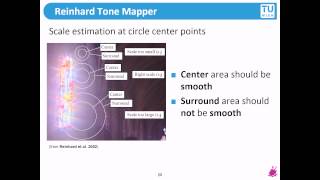
So as I said before, the tone mapper we will look at was developed by Reinhard et al. At Siggraph 2002 presented, so it had already some time to prove itself, so to say it's widely used. So most light simulation products and also HDR photography tools have it. And it has both a global and a local variant, so they were both presented here. You see the difference between a global and a local approach? Yeah. Does it question the local approach? That would be convolutional? Yes, in some way. I mean, usually convolution is by a fixed kernel. So your kernel function is the same here. This could be a nonlinear kernel. So it's not that it's linear convolution in the sense that you have one fixed kernel that does it, but you have a nonlinear mapping in this sense. It's not really convolution, but the implementations are in this period, so if you want to have it fast. So parallelization strategies that work for convolutions also work for that. Usually I will go into the local approach later, but you usually have to adapt the feature size. So either then you do multiple passes with different discretizations of your kernel size, or you take a huge kernel and vary the kernel function. Okay, here the difference between a global and a local approach. I'm not 100% sure how well this is perceivable on this projector, but for example, you see that the local approach has much more contrast in the cupola path, or for example in the in the mosaics on the charge. But the global one already works very well, is faster, but doesn't give you all the possibilities that your eye would give you. So the steps. This is just a short outline. I will explain what is meant with these formulas. Of course, if you want to have in depth details on this, the reference is at the end of the lecture. So here I present the global version. So you now have one mapping function of the whole image, or of the luminance values of the whole image to a color space. So the first thing you do is you compute some kind of average of the image. So since you do not know if this is inherently a very dark image, or is it globally a very bright image, you somehow have to set the baseline, so to say, and this is done with the log average. So you don't just average the the sum, so you don't sum up and divide, because this would give unproportional weight to the large values because they are somehow exponentially distributed. You can imagine. So this takes care of that so you. Average in log space and then convert back into exponential. And then you have some kind of average of your scene. So this is the approximate average brightness of the image that I'm looking at. And then you map this to a middle gray value. So A is now what you define as you want to have middle gray. This you can vary. This also depends on what the range is you have available. And this now sets the bar so everything above this middle gray will be brighter, everything below will be darker. And then. What you do is you take the middle gray value and scale the input accordingly to it. So now you don't have an input in some kind of arbitrary range, but you have it relative to the middle grade value. And then what you do is that you compress the high luminances. So if you remember from before this division by a maximum, which gave you just a single bright spot in the image, this is because the high luminances usually dominate the scene, but are only of very small extent in the scene itself. Imagine looking at the sun. I mean, the sun is very small when compared to the whole sky dome, but it would dominate. It has immensely higher brightness values than the surrounding blue of the sky. So what you do here is now that you map your scale luminance barriers to the final output by compressing the higher luminances. So in the lower right you see the function, the mapping function. So as you see that a huge range, say from value 4 to 10 in the x axis is mapped to a rather small part in the Y axis. That means that a lot of large luminances are just comprised, expressed in a small range in the, say, RGB values. And what you also have is that the small luminance, so the small luminances in the input file or in the input image are mapped to a larger extent on the Y axis. This, you can see that the slope of the function starts out as nearly vertically. At the 45 degree. You have a 1:1 mapping, which is approximately a 2. And then you have a compression. So what this mapping does is it compresses the high luminances and enhances the low luminances. And this then gives you the mapping. And you can convert this into. So I go back. So the output luminances then are in a predefined range from 0 to 1 and can then be mapped to whatever color space you like. So the local version, this is now the one that takes the neighbors into account, starts off similarly. So you compute the log average to get an estimate how is the average brightness of my scene? Then you map the values to average gray. That means that the value of one is now the middle gray that I defined. But now I do not compress the luminance by one uniform function over the whole image. But. But then locally adapt this function by looking at the neighbors. So now. The local average uppercase V now depends not only on the coordinates in the image, so X and Y. So the pixel that I'm there right now, but it also depends on some kind of scale. The scale means how uniform are my brightness distributions. There am I at say, a silhouette where half of it is very dark, half of it is very bright, or am I in a homogeneous region? Because in homogeneous regions your eye would adapt on a larger extent on the retina to this brightness. And if it's accommodated to this brightness, it can differentiate details better. You perhaps have already experienced it when you look at the moon. So if you look quickly at the moon, it's just a bright spot. But the longer you look at it, the more details you can discern in it. This is an adaptation of your eye to it. And this happens also at local spots on the retina. And this is what's simulated here. So you compute for every pixel position XY a local scale. And with this local scale you then you compute a local average V. And this now gives you how much range compression is going to happen at this location. So how to get the scale? So the scale is the extent of an area around this pixel where the brightness does not change too much. So in this example, where you have colorful church window that is illuminated from outside, you have three different examples on how you can put the influence region of your scale. So the Alinehardt Tonemapper does this by computing 2 radii and then look at a certain scale them in a way that they have a certain behavior. So in the very top you see, you assume that the pixel is in the center of the two concentric circles. So this is the pixel that I want to tone map now. And if I lie, if I put two concentric small circles around it, then I see that the center area, the smaller circle, is quite smooth in the distribution of brightnesses. But the outer circle is very smooth too. So there is no significant difference between the small and the large circle. That means that my scale is too small. That means that I could enlarge my circles even more because and still retain smoothness. In the center example, you see the correct application. So the center disk has smooth values, so they are approximately the same brightness. But if you take now the outer circle that intersects the window, you see that suddenly in this footprint, very large brightness values are. So you see that the small circle is smooth, but the surrounding area is not smooth. And this is what you want to achieve when you determine the local scale. The larger the local scale is, the more you are looking at the large patch of equal brightnesses. And your eye would adapt to that. That means that for this pixel, you can improve the contrast because your eye would do the same. Another failure case, what you should not do is that you make the disks too large, as shown in the bottom example. Because here bright values are already in the inner disk. So this scale would be too large. I go back what you get by this. When you know the scale, you know in how large the region is where you can compute your local average. And this then allows you to locally compress your range. So if it's very smooth, you compress less if you're next to very bright boundaries. So if you're next to discontinuities in the brightness in your image, so there are. You are at the verge of traversing from a bright to a dim region, or vice versa, you do the opposite. Yeah, the ratio between the larger radius or smaller is constant. Exactly. Yeah. This is the approach that they take there. And then you have to find this. I mean, they also show you an implementation how this can be efficiently mapped. Because, I mean, trying all the possible circles or disks is not feasible. So you need some kind of approximation that gives you a good estimate on that. Because also if you go to the corner of the image, then some part of this circle is missing. Yeah, I mean, I don't know how they handle this, but I would guess that they just ignore everything that's out of the image. So you have to cope with what you have there. But this is natural. In the corners of your image, you get less neighborhood, so you get less information of how the surrounding looks like. So you will get, say, less optimal tone mapping there. So here another difference. Assume in and the image before. So as you can see, the angel figures on the wall have a much higher contrast. And this is now because the brightness values there are relatively constant. So if you compare this with, say, the window next to it, then this has a very uniform brightness. Even if the colors are perhaps different, this is still a low range. As you saw before, between sun and moon it was 800,000. Between black and white it was 100 or 1,000. So if you have direct or indirect illumination counts much more than just color variations of your surface. So here the dome mapper corrects directly in its local version that the brightness values are quite uniform in this region. So it enhances the contrast. So now this concludes the Reinhardt tone map, but there are also other tone mapping approaches. So in this SIGGRAPH, 2002 was the year of the tone mappers, because there were three tone mapping approaches presented. So one of those was the bilateral filter. Perhaps you already heard of bilateral filtering in computer vision, Perhaps there this is, you can imagine it as a Gaussian smoothing that does not smooth over edges. So if you have a large difference in your image, then it does not smooth this away. So this is, you can also call it edge preserving smoothing. And you can imagine that this is somehow conceptually similar to this scale estimation of a line height, because the scale estimation looks where do the brightness values differ a lot? So, so these are say my brightness edges in the image. And then it doesn't try to propagate contrast enhancement over this edge. And the bilateral filters can do the same thing because they just stop the filtering process at edges. Then another approach by fatal gradient processing, this is, you can imagine an image, say you have only a luminance channel of a single color. Then you can imagine your image as a height function. So bright spots correspond to high peaks, dim regions to low values. And what they do in this work is that they look at the gradients, so how steep are the slopes in my image? And then they compress in gradient range. This allows them to preserve low gradients because these are small slopes are the details in the dimly illuminated regions. And the very high slopes are the ramp ups to the bright spots. So if you just say reduce the high gradients, you also get a similar behavior that you only reduce the range in non uniform regions. So these are three approaches that do approximately the same. They have the same underlying idea, but they have different approaches to it. So one of Reinhard goes more into what's used in photography with darts exposure plates that you can use bilateral filtering immediately uses a well established filtering paraticum in signal processing, but it's most likely very suboptimal from a perceptual point of view. Gradient processing allows a very fast application. But perceptionally, of these three works, the Reinhardt tone mapper is the best. And these speed increases that you perhaps needed 13 years ago are not really relevant now. So you, you don't need to take approximations that were highly relevant before into account anymore and just do the, and just have something that's less efficient but gives you an out of the box nice solution. And if you check Wikipedia, the German version has a longer list. They list approximately 20 different variant. The literature for that is Reinhard not only started that, but also continued research in that. And he's seen as one of the experts to go to when tone mapping is concerned. He wrote a book about that. So high dynamic range imaging. And you can also see these free papers. If you want to know how this field developed, you just check, for example, the Reinhard paper on the digital library of acm. You can do this from here, from the university. So you get an account, you get immediate access to the whole digital library of acm. And there you can just click on cited by. And then you get the long list of papers that referenced the original work by Reinhard. And then you can sort them via years and look what different approaches were used. Good. That concludes the tone mapping part. Are there any questions? Okay, if not, or if you know which method has been used, can we also do vice versa. To some extent? Because I mean, you're inherently losing information. Because, okay, say the thing where you for sure lose precision is if you have before, say 24 bit values and then you encode them in 8 bit RGB values, then you have a quantization of your brightness values. This is unrecoverable, this is just lost. The other thing is if you use local approaches that take the neighborhood information into account and then do different things in different regions of the image, then it could be that you have some kind of ambiguity if you want to reverse this process. Because then it could be that you either had, say in the original data, large brightness values and, and a small scale, or. And a large range compression then. Or the range was already small like that, and you just used less compression. So you do not have the full information how local approaches adapt to certain parts of the image. You will have to infer this somehow, I would guess like an optimization approach. So you would like that locally you should have the same scale that you assume that you reconstruct, and then you can recover your signal, but you will not be able to recover all of it. With global approaches it should be possible. Yeah. Okay. If you combine the global and the local ones, as the reinhardtungbaln does, are they weighted in any way or are equal parts of the global one and the local one? If you look here, the local version has this expression. So the scaled luminance is then divided by some kind of local average and the global version, the first two steps are identical, but then it uses the scaled value only at the very center to, say, compute this local average. So the global version is a special case of the local version that there is not a certain weighting. In the end, you combine a global picture of the local picture or not. No, no, the. No, no, the. The. The luminance output. This is what you get. So for each picture location, you get a scaled luminance between 0 and 1 by the global approach and by the local approach. So here it also immediately gives you the output luminance so that there is no combination going on. Okay, Further questions? Okay, then, thank you for your attention. And this concludes this rendering lecture.