TU Wien Rendering #25 - Path Tracing, Next Event Estimation
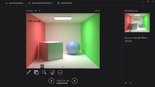
A lecture on path tracing and next event estimation in computer graphics. Covers recursive functions, light sources, and how next event estimation reduces variance in rendering calculations.
Chapters
Let's take a look at how the exact algorithm looks like. I have a recursive function where what I'm looking for first is if I have reached the maximum depth that I would like to render. This means that if I say that I would like to render five bounces, then this is going to be five. Did I reach this number of bounces? Yes. Okay, then just start and return the calibration because this ray is much better than what I'm looking for is the nearest intersection. You remember from the previous lecture that this means parametric equations which I solved for T. So what I'm interested in is that I am intersecting a lot of objects and I'm only interested in the very first intersection. And if I didn't hit anything, then I will return a black color because there's no energy going through this way. Now, if I have the intersection of the object, I will be interested in the emission and the material of this object. Emission means that if this is a light source, then it's going to have emission and the material can be an arbitrary vrdf, diffuse, glossy or some complicated multi layer material. This I'm going to store on N. What's up next? Well, I would like to construct a new ray because I will trace the next ray. So I instantiate a new ray. This will start wherever I hit this object. So if I hit the table, I will create an array that starts from the table and I will set the outgoing direction according to some sampling speed that I have. Let's say that what they have here, if it says that random unit vector in the hemisphere of where the object will sit, and this sounds like a diffuse case to me, So I generate a random unit vector on this hemisphere and this is going to be the outgoing direction. Now let's add together the elements of the random equation. I have the cosine theta, which is the light attenuation. I have the BRDF term. And in the BRDF term it seems that here they have also included this cosine theta part, which is the light attenuation. This is the albedo of the material, how much light is absorbed and how much is reflected. And then what I would like to do is I would call the very same function that you see in line of code number one. So this is a recursive function. I will start the same process again with a new ray, a new starting point and a new direction. And in the end, if I have traced a sufficient number of rays, then I will exit this recursion and I collect the result of this in this variable that's called reflected. And in the end, this is the elegant representation of the rendering equation. The emission, the LE plus the integrated function, which is the BRDF times this reflected, which is all the recursive terms. So this means that I shoot out this ray in the hemisphere and there's going to be many subsequent bounces and I add up all this energy into the reflected incoming light. So this is the pseudo fold. This is not something that you should try to compile or anything like that. But this is what we will code during the next lecture. This is just a schematic overview on what is happening. Exactly. It's actually very trivial. We shoot a ray, we bounce it from the scene, and then we hopefully hit a light source at some point. And even if we hit the light source, we continue. But hitting the light source is important because this is where the emission term comes from. Let me show you what's going on. If we don't hit light sources. So this LE is the emission term on the left side here. So we add this to the end result at every recursion step. And the fundamental question is that if we have a long light path that doesn't hit the light source, we are using completely random sampling or maybe some smart importance sampling. Well then we will never have this emission term. What does this mean? That the radiance that we get from the problem is going to be zero. So the corollary of this is that only you will get radiance. You will get an output from only light paths that hit a light source. If you don't hit a light source, you don't know where the light is coming from. So you will return a black pixel. And this is obviously a really bad thing because you're computing, churning out samples and samples and samples, perhaps on your gpu, but it doesn't return you anything. So it's a very peculiar effect about simple naive path tracing is that if you have a small light source, the convergence of of your final image is going to be slower. Why? Someone help me out. Smaller light sources, more variance, slower convergence because we need a random rays to hit the light source. If it's smaller, then we won't hit it as often. Exactly. Exactly. So the relative probability of hitting the light source is going to be less for a small light source. And up to the extreme where we have a point light source, and if we have a point light source, then we will see that we will be in trouble. Because what I would expect from my path tracer is to return something like this. Well, imagine a point light source in here, but this is not what we will end up with. So I would expect it to return the correct result. Many people have reported to many forums on the Internet that, hey, I implemented it, but this is what I got. Wow, this doesn't work at all. All these Fresnel's law, Snell's law, total internal reflection, Monte Carlo integration for a black image. I mean, I could generate this with five lines of C. Why do we even bother? We will get nothing. Why is that point light source lack image? Why? Yes, exactly. Exactly. So a point. Represents a location. In mathematics, it does not have area. So technically it is the same. Hitting a point light source is impossible because this is the same as what you study in statistics and probability theory, that if you have one number in a continuous scale, what is the probability of hitting this number? Zero. Because that's the point. It has no surface error, it's infinitely small, you cannot hit it. So this is the reason of your black image. If you read the volumes on the Internet, you will find plenty of this. Now we could also sum up our findings Internet beam style, if you will. So if you would like to compute path tracing with a point light source without a technique that is called next event estimation, then you usually will expect a wonderful image. But this is what you will get in reality. Now, the first question is obviously, how do we overcome this? What we can do is that every time we hit something, some object in the scene, be it diffuse or anything, but not light sources, we compute the direct effect of the light source on this point in the scene. So this is a schematic to show what is going on. So I start from the viewer, I hit the speeder, and I don't just start tracing the new ray outwards, but I will connect this point to the light source and I will compute a direct illumination term. This is the schematic for path tracing without the next event estimation. And this is with MaxEvent estimation. So at every station I connect to the light source. In this case, this is actually occluded. In this case, this is debatable. And in the third bounds, you will get some contributions from the light source. Question is, how do we do this exactly? Well, this is the topic. This was the topic of Assignment 0. So the formula that you see in Assignment 0 is exactly the very same thing as what you should be using. What was in there? Well, what we were interested in is there was a term with the 4pi. Because if you have a light source that's A sphere, then what you would. Then we are interested in how much radiance is emitted in one direction. So then you would need to divide by the area of the surface, which is a division by 4pi, and there's going to be the attenuation term, which is R squared, same as in the gravitational law or in the law of electric fields. It means that the further away I am from the light source, the less light is going to be. This is a really good technique because of multiple reasons. And one of the reasons is that you will get contributions from every bounce during the computing the light path. Before I proceed, I would like to tell you that here we are talking about this le, the emission term. And we are adding these parts of this emission term in every bounce. So If I hit P1, I add this something. If I hit P2, I add this something. If I hit P3, then I also add this something. But when I hit the light source, I don't add the emission term anymore because I will be adding it again. So this one L that you would add when you hit the light source by chance. This is distributed into individual properties. Why is this great? One, you can measure point light sources because the direct effect you can actually measure, but you cannot hit the light source itself. So that's great. Two, you will have less variance because it's not like I either hit the light source or I don't. I statistically always will hit the light source unless there are occluders. So I'm adding many samples with small variances, not one sample and lottery, because you either win or you don't get anything. So I can lower the variance, which means that my images will converge faster. And the other thing is that because there are contributions on every bounce, I can separate direct and indirect illumination. So a lot of people do this in the industry, because the movie industry is nowadays using path tracing. I cannot say that like that as a bold, encompassing something statement. But for instance, Disney is now using global illumination in that most important. Why? Because it looks insanely good and it is very simple. And it took them more than 20 years for them to replace their old system, which they really like. It was called gaze. And now they are using global illumination. It has taken a long time, but the benefits of global illumination are now too big to pass on them. And what they are doing is that they get a physically based result. But this is not always what the artists are looking for. Because if you have worked together with artists, then they will say, okay, you have computed a beautiful image, but I would like the shadows to get a bit brighter. You will, as the engineers say, that, well, this is not possible. I computed what would happen in physical reality and that's it. But the artists are not interested in physical reality. They are interested in their own thoughts and their own artistic vision and they would like to change the shadows. So you could technically make one of the light sources brighter and then the shadows would get brighter. But then the artist says, hey, but don't change anything else in the scene, just change the shadows. And then you could pull out your knowledge of the rendering equations that you look, the radiance coming out from this point depends on its surroundings. So you cannot just make something brighter. And the nearby things will also get brighter. You cannot circumvent them. Well, you can. What you can do with the maximum estimation is that you take, you generate an image from the first bounce. So you will get one image which you deposit the radiance that you measured in P1, that's an image. And then you create another image which will only contain the second bounces P2 and upwards. So you would have multiple images and you could technically just add up all of these images with simple addition and you would get physical reality. Great. But if the artist says that I want stronger indirect illumination, then you would grab this buffer, this image that holds up the second and the higher order bounces and you could do some Photoshop or you could do whatever you want with that without touching anything else. So you have a nice separation for direct and indirect illumination. Moving in the street. So moving in the street. They love it. They are playing with it all the time. And later you will see some algorithms that behave differently on indirect illumination and differently directive emulation. You can only do that if you separate these terms. So let's see path tracing. Now with next event estimation, I have the very first bounce. And before I continue my array, I will send the classical, super super classical shadow ray to the light source, randomly chosen point of the light source, and I will add this direct contribution of those light source to this point. And then I continue. Let's go back to the terms. Sorry, we use many terms for the very same thing. This is why I'm writing all of these terms. Because if you read the forums, if you read papers, you will see these terms and they all mean the same. So explicit light, something, maximum estimation, very same thing. So I continue my raid and I also hit the light source with the shadow ray. And then I continue on and on and on. And imagine that this third one is an outgoing ray that actually hits the light source. And if I do, I don't add the L eater in there because I did in the previous process. It's very important to know. Now, you have seen the results for a point light source. Nothing versus something that's pretty hefty. But even if you have a reasonably big light source, like a life light sized light source, I told you that you can have variance suppression effect as well. So this is some amount of samples per pixel. I think it's two, maybe three samples per pixel. So this means that I grab one pixel and I send three rays. So it's three Monte Carlo samples. Now this you can do in two different ways because if you start to use renderers, then you will see how this exactly happens. Some renderers are rendering tiles. So what they do is that they start with some pixels and if you say I want 1000 samples per pixel, then it will start take one or four or whatever number of threads you have on your machine. It will take four pixels and it will shoot more and more samples through it. And after it got to 1000 samples, it will stop and show you a really good and converged pixel. And what we call progressive rendering is the opposite. You pick one pixel, you shoot a ray through it, but only one. And then you go to the next, and then you go to the next. And then you will see an image that has some amount of noise and progressively you will get less and less noise. So this is what you see here is progressive render in motion. Now no next event estimation. So we only get contributions if we hit this light source in the end somewhere. If we don't, we will get a black sample. Now look closely. This is with next event estimation. So there's a huge difference. Such a simple technique can speed up the rendering of many scenes with orders of magnitude faster. You can also play with this program. By the way, this is implemented on Shadertoy, so when you read this at home, just click on the link and play with it. It's amazingly fun.










