TU Wien Rendering #29 - Path Tracing Implementation & Code Walkthrough
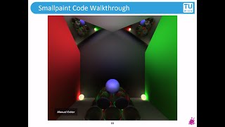
A walkthrough of SmallPaint, a 250-line path tracer that renders soft shadows, color bleeding, and refraction using Monte Carlo sampling. The code covers ray-sphere intersection, recursive tracing with Russian roulette termination, diffuse and specular BRDFs, and Fresnel effects. Student examples show what the implementation produces.
Chapters
What a wonderful day we have today and what a wonderful time it is to write a path tracer. So why don't we get started? What we are going to be looking at is a program called SmallPaint, which is a small path tracer in effectively 250 lines of code. And it contains everything that we have learned during this course. We're going to be able to compute soft shadows, anti aliasing, Monte Carlo integration, and even quasi Monte Carlo sampling, which basically means low discrepancy sampling. This version of the program is going to be able to compute refractions, color bleeding and caustics. And in the end, the binary you compile from the code can be compressed into less than 4 kilobytes. This is how the end result looks like. It has a beautiful painterly look, which actually comes from a bug. And you can also see that the light source up there, the whitish looking sphere, is, you could say, perfectly anti aliased. In order to achieve this with a recursive raytracer and no global illumination algorithm, you would need to compute the very same image on a much larger resolution, then scale it down to a smaller image like this. And this anti aliasing effect you get for free if you compute Monte Carlo path tracing. So the question is, how is this exactly done? And now is the best time to put everything into use that we have learned so far. So let's get started. We have a completely standard vector class. It is a three dimensional vector. It has its own constructor, the classical operators that you would expect. And we also have a dot product for the vector and a cross product for the vector. It is also obviously possible to compute the length of this vector. So nothing too exciting or important here, but we definitely need to build on a solid vector class. Now, the representation of array, array has an origin and a direction. And if you take a close look at the constructor, you can see that when you initialize array with a direction, then this direction is normed. And the reason is that when we compute the dot products between these vectors, most of this information needs to be directional information. So we are not interested in the magnitude of the vector, only interested in the direction of the vector. A good way to get rid of problems where you would initialize your array with directions that are not vectors of unit length. What you can do is to normalize this input in the constructor so you will never have headaches about incorrect results where you have no idea what is really happening. What is the representation of an object? Well, an object has a color. This is denoted by Cl this is actually very sloppy notation. And this you can imagine as albedo, but it is not a double. So it's not a number. It is actually a vector. And the reason for this is the fact that we need to define the albedos. How much light in different wavelengths is being reflected and how much is being absorbed by the given object. Now, objects may also have emission. If they have some non zero emission, then they are light sources. And by type we have an integer that would specify what kind of BRDF we have. It is also important to have an intersection routine and some other function that can compute the normal of the object. Now these are of course virtual functions. We don't define them for an abstract object, but they would have to be implemented in other classes that inherit from the object. Let's take a look at a sphere. So a sphere has this C and R. C is the center of the objects and R is the radius. The constructor is trivial. We have the intersection function. Now you hopefully remember all three of the elements of the quadratic function that we need to solve. But if you take a good look, then you will see that A is missing from here. And the question is why is that? The answer is we are multiplying D with D, the direction vector of array with itself. And if it's a vector that is normed so it is of length one, then this A will always be one. After that we can deal with the discriminant. The discriminant is Normally not B squared minus 4ac. Remember, A is one here, so it's omitted, but it is behind the square root. And this square root is completely omitted here, which looks like a mistake, but it is not. It is essentially an optimization step because you will see that we are testing the discriminant. If it's less than zero, if it's less than zero, then we don't need to deal with this equation because the solutions for the quadratic equation are going to exist in the plane of complex numbers. And that's not a valid T. It's not a valid distance where we would intersect the sphere. If this is not happening, then we can compute the square root for the discriminant. Why after that? Because if the discriminant is bigger than zero, then the square root is not going to make a difference. So what we can essentially do is to postpone the square root calculation after the test. Note that square roots are really, really expensive, so we can save up lots of computational time. If you omit this calculation, there is a really nice Square root hack in the source code of Quake 3, which is by the way, open source. Take a look at how people are trying to hack together functions in order to work better and faster than they should, because square roots are super expensive and there are some really interesting hacks. In order to speed them up, we have the plus and minus term and the division by 2A is again postponed. And that's also another interesting question. Why is this postponed? So you can see that the SOL2 is divided by 2 and the SOL1 is also divided by 2, but only after the test. So it is possible that if we have the solution two, if it is bigger than epsilon, then we have the first expression after the question mark. But if it's not, then we are looking for the second expression after it, which is another test. And if the answer is no for that as well, then we are going to return zero. This would mean that we don't have any hits or the hits are behind us and we are not interested in intersections that are behind our array. There is a possibility that we encountered this, and in this case, I don't want to waste my time by dividing these solutions by two because I'm not going to use them. Why am I splitting hairs here? That's an important question. Why do we need to optimize so much? Because if you grab a profiler, a program that is able to show you in what functions are you spending most of your time in, then this profiler would show you that more than 90% of the execution time is spent in the intersection routines. So you have to have a really well optimized intersection routine. Some programs have replaced these expressions with assembly in order to speed it up even more. So how do we compute the normal of a sphere? Well, very simple. What we have here is P C. Now what does it mean? So if I have A minus B, then this means a vector that points from B to A. So what this would mean, look at the figure here. If I would have a circle, then this would mean that from the center it is pointing towards the given points of the sphere. Now this is also divided by R, because you could imagine you have a sphere that is not of unit radius. And if it's not of unit radius, then this normal vector would have a length. You could compute a normalization. We have a normalized function in our vector implementation, but it also has a square root. So it would be much better to have something that's faster. Well, if you just divide by the radius of the sphere, then you would immediately get a vector of unit length. So in the end we can get the correct result by just simply dividing by R. Excellent. Now we have a perspective camera here. Hopefully you remember from the first lecture we are basically just copy pasting this expression here. We have derived them rigorously and analyzed how this exactly works. A simple intuition. Basically what we are doing, we have as an input an X and a Y. Basically this means give me a pixel with this displacement and what it would give you back is the world space coordinates of these pixels. Uniform sampling of a hemisphere. What is this for? If we are encountering a diffuse object, what we would like to do is to send a ray out on the hemisphere of this object. This we would need to uniformly sample. This means that the Diffuse BRDF is 1 over PI or rho over PI. If you take into consideration the LB dose and you need transforms in order to do it. There is a reading behind this link. How it works exactly is drawing uniform samples on a plane, which is simple, and then we are projecting it on the hemisphere. That's basically all there is. What about the trace function? As you can see here in the first line, this code says that there is a maximum depth. Now clamping after a maximum depth value is not really optimal because whatever number you put in there, the higher order bounces are going to be completely omitted. Now the real solution would be Russian roulette path termination, which we fortunately also have. After depth of an arbitrary number like five, you start the Russian roulette routine which basically says there is a probability for stopping the light path right there. And we generate a random number and compare to this probability. If we don't hit this probability then we will continue our path, but we will multiply the output and the contribution of this light path by this given number that we have specified in one of the previous lectures. So this was implemented by Christian Mahacek and kind thanks. And you can see that later we are going to use this RR factor in order to multiply the contribution of array later. Now what about the intersection routine? This is definitely not the best way to do it, but is sure as hell the easiest way to do it. We specify this T which is going to be the intersection distance, how far we are from the start of the ray and how far is this intersection exactly? ID is basically which object did we hit? And then we iterate through all of the objects in the scene and what we are interested in is calling the intersection routine. This will return a T. How far is the intersection? And what I am interested in an intersection that is the smallest Number this means the closest intersection and also something that is larger than epsilon. Because if I would tolerate zero then this would mean that self intersections are accepted. Therefore every single object that I am on is going to be the first intersection. I'm not interested in this. I know where I am. I just want to know where where I am continuing my path. If there is no intersection, then we return. There is zero contribution where is the intersection in world space. We denote this by hp. This means hit point and where we have started array we traveled along the direction of the ray with this t amount where the intersection is. So this is where we ended up. And the origin of the new ray is going to be this hit point. What is the normal going to be? Well, we just grab the object that we intersected and we are taking the normal with the given function. What is the return radiance? We simply add the emission term. This is the emission term on all three wavelengths. There is a magic multiplier. Disregard that and then we continue evaluating the second part of the rendering equation. The first part is the emission and the second is the reflected amount of light. Let's continue with the inside of the trace function. If we hit an object with a type of one, then this is a diffuse brdf. The next functions compute the next random number for the low discrepancy halton sampler. And the direction is going to be a random sample in the hemisphere. A completely uniform random sample in the hemisphere of this object. What we have Here is this n + the hemisphere function. This is intuition. This is not exactly what is happening. I've just shortened the code slightly in order to simplify what is going on here. The code that you will download will have the real deal in there. Now then we compute the cosine term. Very straightforward. And on the TMP we are going to instantiate a new vector. And this is going to hold the recursion. So the subsequent samples that we shoot out from the hemisphere are going to be added and added to this tmp. Now is the time for recursion. We pass the ray and the scene to the trace function. The ray is actually not the current one is the new one. So basically we set up the new hit point and the new direction of the ray. And this is what we are going to pass to the trace function. We increment the depth variable because we have computed the bounds. The TMP is going to be a variable where we gather all these radians and we put every other parameter that is needed to compute one more bounds. Now the Color is going to contain the cosine term and all this radiance that is collected from the recursion and we multiply it with this CL xyz, which is basically the brdf. So this is the right side of the rendering equation. For a diffuse BRDF, this is multiplied by 0.1. This is just a magic constant. Now, what about a specular brdf? What if we hit the mirror? Well, very simple. We compute the perfect reflection direction. You can see the ray D, and we again set up this variable to collect the radiance in there. And we are not doing anything. We are just going to add the radiance as we get reflected off of this mirror. Then we are going to compute subsequent bounces and, and this is going to be stored on this tmp. So this is what we're going to add to this radiance. What about the refractive material? Well, we have every bit of knowledge that we need for this because essentially this is the vector version of Snell's law. What does it mean? Well, the original Snell's law that we have computed is in one dimension, so it only gives you one angle. But if you are in 3D, you are interested in angles in two different dimensions. This is nothing but the extension of the very same law into higher dimension. Now, where is this implemented exactly? You can see the cosine of theta2. Note that N1 and N2 is considered differently because one of these media is always going to be air. Therefore one of the indices of refraction is always going to be one. The rest is just copy paste. And again you can see that the square root is missing. And we are going to postpone this after the test of cosine T2, because if it is actually not larger than zero, then we are not going to need this variable at all. Therefore we can postpone this after the test. Again, What about the direction of the outgoing ray? Well, this is just copy paste from the formula that we have derived before. So simple as that. Obviously we again need the recursion because if we go inside a glass sphere, then we are going to compute the refraction. So we are going to be inside of the sphere. What does it mean? One, that we have to invert the normal because we are inside, so the normals are flipped. And again we need to compute the trace function, which is the recursion. So we are also interested in the higher order bounces onwards to Fresnel's law. What is the probability of reflection and refraction when rays are bouncing off in different Directions in different angles off of refractive surfaces implemented by Christian Hoffner. So a big thanks for him. It is very simple. You can see that it is exactly the same as what we have learned in mathematics. So this is the R0 term. This is the probability of reflection in normal incidence. And we are interested in the square of that. And note that you don't see the N1 and N2. This is because one of them is always going to be air or vacuum. So it is going to have the index of refraction of 1. Now what about the final probability of reflection? It is also coming from the formula. We have every bit of information we need. So we just put in there this term with the cosine attenuation. How does the main function look like? Well, we have some wizardry with C11 lambda functions, but basically this is just a shortcut. In order to be able to add a new sphere or a new plane to the scene. In one line of code, spheres are given by their radius, position, color. By color we obviously mean albedos, emission and type. Type means what kind of brdf. We have a diffuse, a specular or refractive brdf. Now for planes we have position, normal color emission and obviously type. So what kind of material we have. So using just one line of code, you can add a new object and specify everything, every information that you would need to it. Now we also add the light source and we specify the index of refraction for the refractive BRDFs. And we also specify how many samples per pixel would we like to compute. Onwards to the main loop. We have two for loops that iterate through the width and the height of the image plane. Now vector C is color. It's again very sloppy. What it means is actually the radians that we compute, we instantiate a ray. What is going to be the origin of the ray? This is going to be 000. So this is where the camera is placed. What is going to be the direction of the ray? Well, we connect this ray to the camera plane and we specify which pixel we are computing with I and j. And then we add this weird random number to it. Now what this means is actually filtering. In recursive ray tracing, what you would do is you would only send the ray through the midpoint of a P and that's it. You would compute one sample per pixel. In Monte Carlo path tracing, you're computing many samples per pixel and they don't have to go through the midpoint of the pixel. You would sample the area of the pixel and this Gives you anti aliasing effects for free. If you use it correctly. What is going to be the direction of the ray? Well, this is again the same A, B. The B is the origin of the ray and A is the camera coordinate. So what does it mean? That it is pointing from zero to the camera plane. And we normalize this expression to have array of unit length. Now we obviously call the trace function. The number of bounces is zero. And we pass every information that needs to be known in order to compute these bounces. So we provide this initial ray and the scene and everything else. Obviously we also pass the C and this is going to collect all the radians there is in the subsequent bounces. And then after this recursion is done, we deposit all this energy, all this radiance to the individual pixels and then we divide by the number of samples. Because if we wouldn't do this, then you remember the 1 over n multiplier everywhere in Monte Carlo integration. If you wouldn't do this, then the more samples you compute, the brighter image you would get. And this is obviously not what we're looking for. At the very end we create a file. This is the PPM file format where you can easily write all your contributions in there. We also start a stopwatch in order to measure how long we have been tracing all these rays. So very simple, very trivial. And when we are done, we close the file, it has the image in there and we then write how long the rendering algorithm has been running for. And basically that's it. That's it. This is effectively 250 lines of code that can compute indirect illumination caustics and every global illumination effect and it can compute images like this. This is one student submission from previous years. Absolutely gorgeous. This is the fixed version of Small paint where there are no errors in the sampling. Another one from Michael Kammer. This actually looks like. I don't know if you are into the music band Boards of Canada, but this looks exactly like one of their album covers. Love it. Really cool. And also Sierpinski triangles from Kristian Koestler. You can find the link for the code in there and take a crack at it. Just try it. Build different scenes, try to understand what is going on in there. Try to mess the code up. I wonder what happens if I would not normalize this vector. Play with it. It's a really small, concise and really understandable path tracer. So take your time and play with it. It's lots of fun and you can create lots of beautiful, beautiful images with global illumination. Thank you.










