Andrej Karpathy - Automated Image Captioning with ConvNets and Recurrent Nets
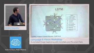
Andrej Karpathy demonstrates how a small LSTM trained on Shakespeare, Linux code, and Magic cards learns to generate text that's sometimes coherent but reveals systematic failures like undefined variables and hallucinated entities. He shows LSTMs dramatically outperform n-grams on structured data, then visualizes what individual LSTM cells learn: quote boundaries, code nesting, if-statement scopes.
Chapters
Okay, so thank you for the introduction. You'll hear about some of the blog posts, by the way, in this talk. I have about 30 minutes, but for the talk, and I have about 110 slides, so I think it's fair to say that I got a little overexcited when I was making the slides for this talk yesterday, and I ended up putting in a lot of really cool and recent work at the end, so I have a whole bunch of slides on this, but I'd really like to just speed through it, and then we're going to get to some of the results that I think are really cool. [FOREIGN LANGUAGE] Okay, so I think most of the talk actually will be about recurrent nets, and so we'll get there in a bit. Now just in terms of very briefly image captioning, so I assume some of you have already seen this work where we take an image and we describe it with a sentence. Most of the models, including mine, rely on two components, a convolutional network that interprets the image and a recurrent network that has really taken place of a language model, and it's predicting the next word in a sequence conditioned on both the previous words and the image information. Now, many of you are presumably familiar with some of the convolutional network work, but I think that recurrent nets are in particular kind of more recent, and so I will spend most of my time on here. So recurrent networks are very nice and flexible models. Normally when you're working with neural networks, you're in this case where you are given a fixed size input and you're trying to produce a fixed size output. So you're essentially learning a function from a domain X to Y. And sequences— and recurrent networks allow you to work with sequences at both input output, or both. And so that's why they are so nice and powerful. And another thing to realize is that even if your input is fixed size, then you can still process it sequentially and take advantage of these powerful models. So a nice example of this is from recent work in DeepMind, where, for example, here they are given a fixed size input, an image, but they process it sequentially by taking a series of glances. And then you string those glances together and you get a sequence, and then you can read out house numbers. And so this network learned a glance policy for starting off in the left and it reads off digits from left to right. So it's quite amazing. It's processing a fixed-size input sequentially. You can also process a fixed-size output sequentially. So in this case also from DeepMind, they are generating digits. So these are all samp— created digits by recurrent network. And the recurrent network is effectively adding canvas to this image over time and creating these digits. So in particular when we do image captioning, we're using a particular type of recurrent network that implements a language model, and in the language model you're just trying to predict the next word in the sequence. And so I have a few slides here on just the basics of how this works, but I'm going to skip through it. We're trying to train a probability distribution over the words in the vocabulary given all the previous words, and so you set up a neural network, and here we put the words here in terms of some vectors that represent every word, and then the targets always are the next word, and these are just targets, and these are all softmax classifiers. This is all just a cross-entropy loss, and we backpropagate it and train this over time. At test time, the way this works is we have a probability distribution over the next word. We start off with a special start token. We get a probability distribution over the first word. We sample from it, then we put the representation of the sampled word on the bottom, and we forward and sample, forward and sample, and we continue doing this until we get a special end token as the sampled token, and then we halt the generation. That's just the language model, but if you're trying to generate images, or describe images, then, not generate images, just describe them. Then we basically have an image and a sentence, and the way this works is that we take the image, we pass it through a convolutional network, but we're going to get rid of the softmax classifier, and instead we're going to redirect the representation into a recurrent network, and here we have just a standard language model, but we're conditioning it through this interaction on the image information as well. And so this y0, we'd like that to be straw, y1 we'd like to be hat, and y2 we'd like to be the special end token. So we can train that with backpropagation, and then at test time we take an image, forward it through the ConvNet, redirect the representation into the recurrent net, and then sample words one at a time until we special end token, until we sample special end token, and at this point we've described this image as a straw hat, period. And so we train these datasets on image sentence, we train these networks on image sentence datasets, and then we get some results. So some results work really nicely, and you've seen a lot of examples of these, so I won't spend too much time. So some work really nice, some work kind of okay. So I mentioned some of these in my oral, and some of them don't work quite well. Maybe there's a horse standing in the middle of a road. Not really. But basically you end up creating sentences for images, and there's a whole bunch of work on improving on these models and pushing them further. Okay, so this was about half a year ago for me, and when I was looking at these results first, and I was getting these results out of recurrent network sampling these words, I thought that these were fairly impressive results, and I wasn't really used to seeing something like that come out of a simple model like that. And— but what I learned since then as I've applied recurrent networks to different problems is that these results are in fact quite reasonable in the sense that the recurrent network only has to model a sequence of about 5 to 10 words, and, you know, basically what it ends up doing is it learns some kind of templates, like noun in noun is verb in noun, and then it fills them in based on the content of the image and based on the textures that it sees in the image. And so we're not really pushing this too far. We're 5 to 10 words and we're filling it in. And so some of the models that— I discovered that there are a lot of tasks where the performance seems quite unreasonable of these models. And so this became the title of my blog post that I published about 2 weeks ago, and so you can check it out on karpathy.github.io. I'd like to briefly show you some of those results that I believe are kind of unreasonable and not clear what's going on, and then the later part of my talk is about trying to understand what is going on and how it comes about. In particular, we're going to be working with character-level language models. We're still trying to predict the next thing in a sequence, but now it's not words, but it's characters. Characters are nice because it's a very nice and interpretable testbed. We can inspect them and we can work with them, and there's a lot of datasets and and so on. And so we assume some particular vocabulary, for example, and then if we have a training sequence, then we're going to set up the characters over there, and then we have some target characters, and then we train this with backpropagation. And so we're going to train character-level sequence models. The input is always just a long sequence of characters, and we're trying to train the probability distribution to predict the next character in the sequence. So some of the datasets that I first fed into these networks when I was starting to work on this, for example, are Shakespeare. So I took Shakespeare, you take all of the works of Shakespeare, all the sonnets and plays, and you concatenate it all into a single file. It turns out to be about 3 megabytes. And then you train a character-level sequence model on these characters, and then what you can do is you can sample from the model one character at a time. And what you find is that the model makes quite reasonable-looking poems. And so first thing to note, of course, is so this model discovers things like words and it learns to spell them. It doesn't make too many spelling mistakes. It knows how to use spaces and commas, and all of this is sampled, including the names of these people, and it uses quotes, and it puts periods at the end of sentences, and it does a lot of really quite reasonable things, and the gestalt of this is quite— quite good. Now, when you actually look at the semantics, it doesn't always look that good, but we're going to go into that in a bit. Now, we tried to push these results, and we tried to go into more difficult domains, so a friend of mine, a labmate, Justin Johnson, has looked in particular on— the Stacks project. This is a collaborative project from mathematicians, and they're writing an algebraic topology book. And so you can download the LaTeX file. I believe it's a couple tens of megabytes of LaTeX, and you can just train a character-level language model on this, so we can then sample LaTeX. And so this is sampled mathematics. We sample this a character at a time. Now when you first actually create this, it doesn't compile right away, but then you go into the LaTeX and you try to fix some of the mistakes. It doesn't take too long, and then you can compile it. Some of the mistakes, by the way, that it makes, just to give you a sense, is it begins an itemize environment but then it closes an enumerate environment and stuff like that. So sometimes it forgets exactly what environment it's in, but in terms of spelling mistakes, those are very rare. And so, you know, there's math here. It looks— I can't distinguish it from the actual book. Sometimes it tries to generate diagrams as well, but of course if you're familiar with the syntax, you know that that's very difficult to actually model in terms of the— how you specify that in LaTeX. My favorite part is that proof on top is omitted. So the recurrent network just did not feel like filling that proof in. But otherwise, there's very few mistakes. It comes up with all kinds of lemmas and corollaries, and you can sample just infinite number of algebraic topology. So we wanted to push this further, and I was really curious about what is the most structured, most difficult dataset that you can plug into a recurrent network? And so my answer to that was code. And so in particular, I looked at Linux. On GitHub, you can download all of source code of Linux. It's about 600 megabytes. You concatenate all the source file, all the header files into a single giant file, and then you train a character-level recurrent network on it. You let it train for overnight and you come back in the morning, and then you can sample code. And so the character-level RNN, knows quite a lot. When you look at the gestalt of this, it's very good. So it creates a function. It takes some arguments. It creates some variables. It can indent code. It samples spaces and tabs over here, and it knows how to count them. It closes ordered braces. It puts some comments in there. Comments its own code. So, you know, quite indistinguishable. When you look at some of the mistakes that it makes, by the way— [Speaker:MAN] File? Almost absolutely not. So what's funny about this is it takes some variables, m and v, but then it doesn't use them. That's, for example, or it sometimes uses variables that were not declared. For example, here it's a void function and it doesn't return, so that's a nice long-term dependency, but I don't think that this is something that happens very consistently, so sometimes that's something very long-term that might not happen all the time. A slightly amusing thing about this is that Linus Torvalds, the chief architect of Linux kernel, he thought that this was really amusing, so he shared this on Google+. And he's not a fan of traditional AI and rule building and Lisp, Prolog, and so on, but he's just waiting for neural nets to take over. So this post convinced him, and he thought that this was really funny. Now what's really amusing about this is when you look at this model just sampling over time, and it's just spewing out infinite amount of code. Like in front of you in the console. And what's really funny is that sometimes the model decides that it's time to start a new file, and that's the most amusing part for me. Because when it samples a new file, the first thing it does is it recites the GNU GPL license character by character. Okay? It's perfect. And the reason it knows this by heart is because it occurs in many files, so it just learns it by heart. And then it's like, okay— [Speaker:AUDIENCE] How big is your model? [Speaker:ANDREJ KARPATHY] Sorry? [Speaker:AUDIENCE] How many parameters in your model? [Speaker:ANDREJ KARPATHY] This was a 700-unit LSTM with 3 layers. So the number of parameters is about 5 million. 3 million, something like that. Okay, so it sampled the GNU license, then it goes on for some includes, then it samples some macros, and then it dives into code. And so it has this notion of very long-term evolution of a source file in a codebase. And so I thought this was quite impressive when we were looking at this. By the way, I also published the codebase for all of this, so it's called Andrej Karpathy. It's on GitHub. And so you can all play with this. It's written in Torch. And so the input to this is really one giant text file, and you just let it— leave it train, and then you can sample character-level stuff. Just to give you an idea, by the way, a lot of people have played with this since I've released this about 2 weeks ago, and a lot of really fun things. So people trained it on books of cooking recipes. So here's a sampled recipe, and this is for a basic cheese wings. And it's a dessert, and it makes 6 servings, and you need a whole bunch of stuff, and the way you make it is you preheat the oven to 350°F, and you combine sugar, salt, baking soda, celery, and sugar. You add the chicken broth. Well, and then you add cornstarch to the pan, you cool, you add olive oil and cooking spray, and then you pour onions until melted, and you're done. So that's how you create a— cheesy cheese wings. Now some of the funny things here are, again, we're coming across the same high-level themes as we're coming across when we looked at the code. It declares all kinds of things that you need for this recipe and then doesn't use them, and it also uses all kinds of things that it didn't declare, so these are some of the longer-term interactions. Also what's interesting is that, for example, it lists sugar twice. So these are some of the higher-order patterns that you will not find these recurrent networks making. So you and I know that when we're enumerating a list, it doesn't make sense to actually list an ingredient twice when you're you're about to combine it, but it actually lists them twice because it doesn't know about this higher-order pattern. It cannot generalize across that so easily. It just has this notion of ingredients, and then it knows that it should be sampling a new ingredient after a comma, but it doesn't really have this capacity to think about these higher-order patterns. People have also run it on Obama speeches, and there's a whole bunch of funny things about men and women in military uniforms and so on, but the parts I like is that it greets them. Greets very nicely, good afternoon, God bless you, and it ends very nicely, thank you very much, God bless you, and God bless the United States of America. And so it learns these phrases by heart because they just occur at the end of speeches very often. People have also trained it on the Bible, so there's a Char RNN Bible bot, and so this is just sampling things. It's about the Lord and I don't know. I don't think that this is a very well-trained model, but it's still hilarious. Sometimes. Another thing that people have tried is there's this ABC notation where you can express music, and so you just feed this into the RNN and then it can sample music and you can listen to it. I don't have it with me here, but what's also amusing about this is it's fairly nice. You can listen to it. I link to it from the blog post. What's nice about this is that the titles are also in the description, and so when it samples this music, then it also calls its own— it makes up names for its own masterpieces. So this masterpiece here is called Lisslstis, and you can listen to it, and it's completely made from an RNN. Another one is NSF abstracts. Turns out there's a dataset of 400 megabytes of NSF abstracts, so this is a sampled NSF abstract, and what's funny about this— okay, so this is about an integration— integration diffusivity in mechanisms of processing and minimal components in central topology, and So what's interesting about this, it knows that date is followed by date-like things. It knows about digits and numbers. And the sponsor, where is this? Oh, the investigator, Jennifer Störslund, and I don't know. I tried to look up this person, but they don't exist. So this is just completely hallucinated information for the most part. And so yeah, you can read through these abstracts, infinite abstracts, NSF abstracts, and I'm curious if they would actually go through the process that would be funny. Another thing is people have tried to get this around with Magic cards, and so there's a huge database of Magic cards, and then people really love this on the forums, so they started to create, like, concept art and embedding these, like, sample things and just making up these cards, and they want to play with this, so this would be quite hilarious. Okay, so I've shown you a wide array of how people are playing with this, and that's all fun and nice to look at. But I think one of the more constructive responses to my blog post was from Yoav Goldberg, and in particular he was thinking about, this all looks impressive, but let's just step back and let's just see how far you can go with finite context. In particular, if you train a 10-gram model, how far can you go? And so, for example, he trained a 10-gram model on Shakespeare, so that means that you're only giving yourself the last 10 characters and then you have a distribution over the 11th. And so what he found is that this Shakespeare actually looks relatively indistinguishable from the LSTM. You can't really tell the part very easily. But when you take a 10-gram model and you try to run it on Linux, then everything completely breaks. And so this model cannot keep track of spacing. It cannot— it does not close any of these brackets and so on. So some of these datasets are basically much more impressive than others. In particular, Linux is an extremely difficult dataset. [Speaker:AUDIENCE] Is this space or character limited? [Speaker:ANDREJ KARPATHY] Sorry? [Speaker:AUDIENCE] Is this space or character limited? [Speaker:ANDREJ KARPATHY] It was both. It was weird. It's weird. Yeah. And so we agreed with Yoav in that something very interesting was going on in terms of these results, and we wanted to understand this as much as possible. And so this inspired our most recent work. It's called Visualizing and Understanding Recurrent Neural Networks. It's now on arXiv as of about 4 days ago. And we really tried to drill down and understand how these models can perform such complex tasks. And this is done in collaboration with my labmate Justin Johnson. We are equal co-authors on this paper. And my advisor Fei-Fei Li. And so in this work, we worked on deep recurrent neural networks. So here, for example, we have a 3-layer RNN where you set up the characters again on the bottom, and we have targets on the top. I don't think I have— so not only do we work with RNNs, but also with LSTMs, because LSTMs always work better. Now, LSTMs look very scary when you look at them for the first time. I think this diagram only makes sense to you in retrospect. I already understand LSTMs very well, and now it makes sense, but I remember first time seeing it about 4 months ago, it was complete nonsense. The way I like to look at LSTMs is just in terms of the equation. It's not that scary once you look at this. You have a few input forget output gates, and you basically have the cell state, which is like a memory. The best way to think about an LSTM is kind of like a class. It has its own internal variables. That's the cell state, c, and then it can learn. It can forget a variable. It can rewrite a variable or add some value g to it, and it can also reveal some of its hidden, hidden state to the layer above or after. And so that's gated by this output gate, and it reveals the tanh of its memory to outside. And so h is really what governs the behavior afterwards. So c is an internal variable. That's one way to look at it. And so we can forget a variable, we can add to it, and we can reveal it, and that's gated by these binary gates, but we make them sigmoidal so that the model is trainable, because otherwise if you have binary gates, you cannot train this with backprop because there are no gradient. And so in terms of the datasets that we used, we tried to look at the two extremes of structure-ness. So we looked at some English novel, in particular we used War and Peace because it's a huge book, and we looked at Linux kernel because that's a very difficult and structured dataset. And so we wanted to train a whole bunch of models, n-gram models, RNNs, and so on, And so just to give you— I'm not going to go through all of this, of course, but n-gram model here is a strong n-gram baseline. We're using Kneeser knee smoothing and KenLM, which is a very popular package for creating n-gram models. We train n-gram models up to 20. We get some loss, so low is good. Then we train some recurrent networks, and we control for parameter sizes very carefully. And I don't have time to go into all the takeaways here. Just note that the recurrent networks perform better than those n-gram models. But one thing to note here is that these are actually fairly small recurrent networks. These are only 1.5 million. So our checkpoints are 11 megabytes, and those checkpoints are 3 gigabytes. So this is a very efficient, tiny model that performs better. And we're not really trying to compete with n-gram models. That's not the point. What we're trying to get at here is we're trying to squeeze out as much juice as possible from the last n characters because that allows us to somewhat get an understanding of how long are the interactions in the LSTMs. And so in particular, this here suggests that maybe they're longer than 20. By some amount. But of course this is not very informative, so we try to dig deeper, quite a bit deeper. So in particular what we do is we look at all those errors that we're making on the test set, and we try to categorize them by the characters that they occur at. And so the question really we're asking is, what characters do LSTMs perform much better on, or which characters do n-gram models perform better on? And so we're going to look at the probability of getting the character correct, like the mean probability of getting a character correct as a function of the character. And so when we look at this on the Linux dataset, what we find here is elistims are in red. So these are all characters where the elistim performs quite a bit better, and over there we have characters that the 20-grams do slightly better. And so what we find is that on the Linux dataset, the elistim performs much better on all these special characters— braces, semicolons, tabs, all the brackets, basically. Uh, we're outperforming n-grams by quite a bit on those characters. And on the other characters, we're losing out a tiny bit. Now, I don't know exactly how to justify the loss on the other characters. I think basically the Austrians are quite small. 1.5 million is quite small. And you have a finite amount of capacity to learn this dataset. And so the LSTM probably just allocates that capacity to keeping track of the brackets instead of the other characters. And it ends up losing out on them a tiny bit. In terms of War and Peace, what's interesting is, again, a similar story where we outperform the 20-gram by a lot on /r/. This is a carriage return character. It's a new line. I'll show you this in a bit. I'll come back to this War and Peace result, but for now, for Linux, we saw that the closing brace is something we do quite a bit better on. And the closing brace is something that we can actually try to understand even deeper, in a sense that we can look for the opening brace backwards in the text, and we can try to find how far in the back is the opening brace in the cases where we get the closing brace. So that gives us an idea about how long is the interaction the LSTM can keep track of. And so here we're looking at the distance of the opening brace to the closing brace, and we're looking at the advantage of the LSTM over the n-gram model on the closing brace character. And so what we're finding is that when the distance is about 0 to 10 characters, then the LSTMs don't perform much better than the n-gram models. But once that distance starts to climb, then we start to gain a huge amount of improvement. And so— and at some point it's gets interesting at about 60. We start to go down and we start to level off. And so what this seems to suggest is that maybe the dependencies are roughly on the order of 60 characters. We keep capturing more and more brackets in— with respect to the n-gram model up to about 60. Another kind of interesting kind of experiment that we tried to look at is in terms of the actual representation of the LSTM. So in particular, this is the cell state. That's the internal memory. and what we can do is we can visualize that cell state for some cell in the LSTM as we are reading the text. So this is some test set text, and the LSTM is reading through, and I picked a particular cell in the LSTM, and I'm just visualizing its activation. So this is kind of like neuroscience but with an LSTM. We're just trying to look at the firing rate of this cell neuron as we're reading this text. And so I'm coloring red as -1 and blue as +1, and 0 is white. and so we can see where the LSTM gets excited— the LSTM cell, this particular one, gets excited. And so most of these are kind of unintelligible, kind of like this one. It's not really quite clear what's going on. But then you start going through them, and we went through quite a bit at the end, and it doesn't take too long before you start to discover some cells that are actually quite interpretable. So for example, on War and Peace, we find cells that turn on when there's a quote, and then turn off at the end quote. So, these cells very robustly just turn on whenever you are inside a quote environment. That's one interesting type of cell. Now, something to keep in mind when I'm going through these results, by the way, is the way we train these models is we, of course, don't backpropagate through the entire sequence. We do finite backpropagation through time in 100 steps because you can't afford to go too far to the back. In terms of backpropagation and gradient flow, the LSTM can only notice dependencies of up to 100 steps. 100 characters. And so it's interesting that this dependency here is much longer than 100, but the LSTM still learns it. And so the fact that this works, basically the only explanation that we know of is that whenever you see quote patterns that are shorter than 100, the LSTM learns that pattern, that it's useful to keep track of whether or not you're in a quote because someone is saying something, and then it generalizes to above 100. And so this one is above 100 and it seems to generalize. Another kind of interesting cell that we found was one that very robustly keeps track of the line length. So here, very interpretable when you look at the input, the forget, and the output gates. It's quite amazing. It basically starts off at 1. When it reaches— and it slowly decays the cell. And when it gets to the end, it resets to 1. And then it just does this all the time. And so it's some kind of a line-tracking cell. Now, something to note is remember that in this diagram we saw a huge amount of advantage for the carriage return when you're predicting your line. The LSTM can do this much better than a 20-gram model. You might imagine that a cell like this that decays over time would be very useful because usually in this dataset these newline characters come in roughly after 70 characters. This LSTM cell just keeps track of how far down the line you are, and then that can probably predict this quite well. Another cells we found is cells that turn on inside if statements quite robustly, and this is for Linux. Cells that turn on inside quotes. Quotes and also comments and turn off everywhere else. So the LSTM can use these cells to know whether or not it's just writing out text or if it's actually coding. Another kind of cell that we found that is interesting— oh, by the way, there's also cells for just quotes, just comments but not quotes. This one also responds to quotes. We also find cells that are very sensitive to depth of the statement in Linux code. So whenever you start to nest statements, then it will just start to turn on more and more. It's kind of an interesting dependency. And then you find all kinds of other cells that seem interpretable, but it's not quite clear what they're for. So this one, for example, it turns on at the end of the statement in some very funny way, but it doesn't just turn on for every semicolon or every bracket, because there are lots of brackets inside here where it doesn't turn on. It just kind of, like, turns on at a matching bracket. So it might be predicting a newline character. We're not actually quite sure. I've shown you a lot of— we're drilling down to see what kinds of dependencies we're capturing that n-gram models are not capturing. We've gone through some visualization experiments. These are impressive but final model checkpoints. These models have been trained for quite a long time. We asked the question of how does this develop over time? What are the learning dynamics of these LSTMs as you train them? What we can do, for example, just qualitatively, is we can look at training iterations, so these are all different checkpoints at different amount of time as the LSTM is training, and we can sample text. And so this model has only seen a couple of training iterations, just a few tens of thousands of characters, and you can see that it's mostly gibberish, but it's already starting to use the space character a tiny bit and so on. And then over time it starts to put together these words. It starts to then learn words like we and to and his. You start to see some short words. And then you start to see longer words like fall and unsuch— that's not a word, but— that and hall and prince. So already we're starting to see some longer things, and eventually just all words. And so what's interesting qualitatively is that it kind of seems to build it out from small out. Like, you start to learn from inside out every one of those words, from shorter to longer. And we can quantify that more precisely. —in terms of— so what we do here in this experiment— how much time do I have left, by the way? 5 minutes? OK. I should leave some time for questions. So just very briefly, we can look at how different your predictions on the test set are from n-gram models in terms of KL divergence, symmetric KL divergence. And what we find is that as you train the LSTM, we become very similar to 1-gram models, and then we diverge, and then to 2-gram models, and then we diverge, and then 3-gram models, and then we diverge, and then 4-grams. Basically, this seems to hint that we're learning from 1-grams out, and then we just don't stop until very long dependencies. This is actually relevant if you're trying to design some of these systems. I don't want to go into too many details, but for example, the machine translation system from Oriol and Ilya and so on, they had to split the source sentence to get it to work very well, and that's— Okay, I can't go into it. Sorry. But basically, this informs some of the design decisions when you're actually trying to come up with this. You don't want to give the LSTM just long-term dependencies right away. You want to give it a chance to grow out its dependencies over time. I think we have a lot of error analysis that we're trying— We're trying to figure out what are the limitations of LSTMs, and so what we do is we peel errors one by one, and we're trying to get an understanding of the error breakdown in terms of the errors. Just very briefly, one interesting error is— Suppose that this sentence is in your test set. John yelled at Mary, but Mary couldn't hear him. What we found is that what's interesting is if the LSTM doesn't get this word Mary, so it makes mistakes, it mispredicts on M, A, R, and Y, it mispredicts on those, then what you find is that almost always it is the case that it mispredicts in exactly the same ways on the second Mary as well. You might think that this is kind of odd because the LSTM could, you might suppose that it could keep track of the previous context because the occurrence of Mary here should make the occurrence of Mary just a few characters down the road much more likely, but something like this doesn't seem to be happening. If you think about it more, this is another example of this kind of a higher-order pattern where the LSTM can't just learn that, okay, for any characters, for any characters sequence that happened in the past, I'm going to try to replicate it if it ever comes up in the future, something like that. These higher-order patterns are not being used. All that's going on is kind of this memorization and a few kind of interesting cells. We have a lot of this error breakdown and how this differs between big LSTMs and small LSTMs, and it's very interesting. I encourage you to check out the paper. And so the conclusions are LSTMs are very powerful models. We still haven't really understood how they work, but at least we tried with one paper. And we have some interesting experiments that support that there are interpretable cells, long-term dependencies, and we can find them, and we can start to understand how they work. And some limitations based on the inner analysis that I didn't have time to go into. But basically, very powerful models, and I'm looking forward to the future with these models. Thank you.
More from Andrej

Skill Issue: Andrej Karpathy on Code Agents, AutoResearch, and the Loopy Era of AI







Andrej Karpathy: Tesla AI, Self-Driving, Optimus, Aliens, and AGI | Lex Fridman Podcast #333