Building makemore Part 4: Becoming a Backprop Ninja

Andrej Karpathy derives and codes the backward pass for batch normalization by hand. He works through the calculus to get gradients for μ and σ², simplifies the result into one line of PyTorch, and validates it against autograd with differences around 1e-9.
Chapters
Hi everyone, so today we are once again continuing our implementation of Make More. Now so far we've come up to here, multilayer perceptrons, and our neural net looked like this, and we were implementing this over the last few lectures. Now I'm sure everyone is very excited to go into recurrent neural networks and all of their variants and how they work, and the diagrams look cool and it's very exciting and interesting and we're going to get a better result, but unfortunately I think we have to remain here for one more lecture. And the reason for that is we've already trained this multi-layer perceptron, right? And we are getting pretty good loss. And I think we have a pretty decent understanding of the architecture and how it works. But the line of code here that I take an issue with is here, loss.backward. That is, we are taking PyTorch autograd and using it to calculate all of our gradients along the way. And I would like to remove the use of loss.backward, and I would like us to write our backward pass manually on the level of tensor. Tensors. And I think that this is a very useful exercise for the following reasons. I actually have an entire blog post on this topic, but I like to call backpropagation a leaky abstraction. And what I mean by that is backpropagation does— doesn't just make your neural networks just work magically. It's not the case that you can just stack up arbitrary Lego blocks of differentiable functions and just cross your fingers and backpropagate and everything is great. Things don't just work automatically. It is a leaky abstraction in the sense that you can shoot yourself in the foot if you do not understand its internals. It will magically not work or not work optimally, and you will need to understand how it works under the hood if you're hoping to debug it and if you are hoping to address it in your neural net. So this blog post here from a while ago goes into some of those examples. So for example, we've already covered them, some of them already. For example, the flat tails of these functions. And how you do not want to saturate them too much because your gradients will die. The case of dead neurons, which I've already covered as well. The case of exploding or vanishing gradients in the case of recurrent neural networks, which we are about to cover. And then also you will often come across some examples in the wild. This is a snippet that I found in a random codebase on the internet where they actually have like a very subtle but pretty major bug in their implementation. And the bug points at the fact that the author of this code does not actually understand backpropagation. So what they're trying to do here is they're trying to clip the loss at a certain maximum value. But actually what they're trying to do is they're trying to clip the gradients to have a maximum value instead of trying to clip the loss at a maximum value. And indirectly, they're basically causing some of the outliers to be actually ignored because when you clip a loss of an outlier, you are setting its gradient to 0. And so have a look through this and read through it, but there's basically a bunch of subtle issues that you're going to avoid if you actually know what you're doing. And that's why I don't think it's the case that because PyTorch or other frameworks offer autograd, it is okay for us to ignore how it works. Now we've actually already covered autograd and we wrote micrograd, but micrograd was an autograd engine only on the level of individual scalars. So the atoms were single individual numbers. And, you know, I don't think it's enough. And I'd like us to basically think about backpropagation on the level of tensors as well. And so in a summary, I think it's a good exercise. I think it is very, very valuable. You're going to become better at debugging neural networks and making sure that you understand what you're doing. It is going to make everything fully explicit. So you're not going to be nervous about what is hidden away from you. And basically in general, we're going to emerge stronger. And so let's get into it. A bit of a fun historical note here is that today writing your backward pass by hand and manually is not recommended, and no one does it except for the purposes of exercise. But about 10 years ago in deep learning, this was fairly standard and in fact pervasive. So at the time, everyone used to write their own backward pass by hand manually, including myself, and it's just what you would do. So we used to write backward pass by hand, and now everyone just calls loss.backward we've lost something. I wanted to give you a few examples of this. So here's a 2006 paper from Geoff Hinton and Ruslan Selakhtynov in Science that was influential at the time. And this was training some architectures called restricted Boltzmann machines. And basically it's an autoencoder trained here. And this is from roughly 2010. I had a library for training restricted Boltzmann machines. And this was at the time written in MATLAB. So Python was not used for deep learning pervasively. It was all MATLAB. And MATLAB was this scientific computing package that everyone would use. So we would write MATLAB, which is barely a programming language as well, but it had a very convenient tensor class. And it was this computing environment, and you would run here. It would all run on a CPU, of course, but you would have very nice plots to go with it and a built-in debugger, and it was pretty nice. Now, the code in this package in 2010 that I wrote for fitting researchable submachines to a large extent is recognizable, but I wanted to show you how you would— well, I'm creating the data in the XY batches. I'm initializing the neural net. So it's got weights and biases just like we're used to. And then this is the training loop where we actually do the forward pass. And then here at this time, they didn't even necessarily use backpropagation to train neural networks. So this in particular implements contrastive divergence, which estimates a gradient. And then here we take that gradient and use it for a parameter update along the lines that we're used to. Yeah, here. But you can see that basically people were meddling with these gradients directly and inline and themselves. It wasn't that common to use an autograd engine. Here's one more example from a paper of mine from 2014 called "Defragment Embeddings." And here what I was doing is I was aligning images and text. And so it's kind of like CLIP, if you're familiar with it, but instead of working on the level of entire images and entire sentences, it was working on the level of individual objects and little pieces of sentences. And I was embedding them and then calculating very much like a CLIP-like loss. And I dug up the code from 2014 of how I implemented this, and it was already in NumPy and Python. And here I'm implementing the cost function, and it was standard to implement not just the cost but also the backward pass manually. So here I'm calculating the image embeddings, sentence embeddings, the loss function. I calculate the scores. This is the loss function. And then once I have the loss function, I do the backward pass right here. So I backward through the loss function and through the neural net, and I append regularization. So everything was done by hand manually, and you would just write out the backward pass, and then you would use a gradient checker to make sure that your numerical estimate of the gradient agrees with the one you calculated during backpropagation. So this was very standard for a long time, but today of course it is standard to use an autograd engine. But it was definitely useful, and I think people sort of understood how these neural networks work on a very intuitive level. And so I think it's a good exercise again, and this is where we want to be. Okay, so just as a reminder from our previous lecture, this is the Jupyter notebook that we implemented at the time, and we're going to keep everything the same. So we're still going to have a 2-layer multi-layer perceptron with a batch normalization layer. So the forward pass will be basically identical to this lecture, but here we're going to get rid of loss.backward, and instead we're going to write the backward pass manually. Now here's the starter code for this lecture. We are becoming a backprop ninja in this notebook. And the first few cells here are identical to what we are used to. So we are doing some imports, loading the dataset, and processing the dataset. None of this changed. Now here I'm introducing a utility function that we're going to use later to compare the gradients. So in particular, we are going to have the gradients that we estimate manually ourselves, and we're going to have gradients that PyTorch calculates, and we're going to be checking for correctness, assuming of course that PyTorch is correct. Then here we have the initialization that we are quite used to. So we have our embedding table for the characters, the first layer, second layer, and a batch normalization in between. And here's where we create all the parameters. Now you will note that I changed the initialization a little bit to be small numbers. So normally you would set the biases to be all zero. Here I am setting them to be small random numbers, and I'm doing this because if your variables are initialized to exactly zero, sometimes what can happen is that can mask an incorrect implementation of a gradient, because when everything is zero, it sort of like simplifies and gives you a much simpler expression of the gradient. Than you would otherwise get. And so by making it small numbers, I'm trying to unmask those potential errors in these calculations. You also notice that I'm using, uh, b1 in the first layer. I'm using a bias despite batch normalization right afterwards. So this would typically not be what you do because we talked about the fact that you don't need a bias, but I'm doing this here just for fun because we're going to have a gradient with respect to it and we can check that we are still calculating it correctly even though this bias is spurious. So here I'm calculating a single batch, and then here I am doing a forward pass. Now you'll notice that the forward pass is significantly expanded from what we are used to. Here the forward pass was just, um, here. Now the reason that the forward pass is longer is for two reasons. Number one, here we just had an F.cross_entropy, but here I am bringing back an explicit implementation of the loss function And number 2, I've broken up the implementation into manageable chunks. So we have a lot, a lot more intermediate tensors along the way in the forward pass, and that's because we are about to go backwards and calculate the gradients in this backpropagation from the bottom to the top. So we're going to go upwards, and just like we have, for example, the logprops tensor in a forward pass, in the backward pass we're going to have a dlogprops, which is going to store the derivative of the loss with respect to the logprops tensor. And so we're going to be prepending d to every one of these tensors and calculating it along the way of this backpropagation. So as an example, we have a b and raw here. We're going to be calculating a db and raw. So here I'm telling PyTorch that we want to retain the grad of all these intermediate values because here in exercise 1, we're going to calculate the backward pass. So we're going to calculate all these d variables, and use the cmp function I've introduced above to check our correctness with respect to what PyTorch is telling us. This is going to be exercise 1, where we sort of backpropagate through this entire graph. Now, just to give you a very quick preview of what's going to happen in exercise 2 and below, here we have fully broken up the loss and backpropagated through it manually in all the little atomic pieces that make it up. But here we're going to collapse the loss into a single cross-entropy call and instead we're going to analytically derive using math and paper and pencil the gradient of the loss with respect to the logits. And instead of backpropagating through all of its little chunks one at a time, we're just going to analytically derive what that gradient is and we're going to implement that, which is much more efficient as we'll see in a bit. Then we're going to do the exact same thing for batch normalization. So instead of breaking up batch norm into all the little tiny components, we're going to use pen and paper and mathematics and calculus to derive the gradient through the BatchNorm layer. So we're going to calculate the backward pass through BatchNorm layer in a much more efficient expression instead of backward propagating through all of its little pieces independently. So that's going to be exercise 3. And then in exercise 4, we're going to put it all together. And this is the full code of training this 2-layer MLP. And we're going to basically insert our manual backprop and we're going to take out loss.backward, and you will basically see that you can get all the same results using fully your own code. And the only thing we're using from PyTorch is the torch.tensor to make the calculations efficient. But otherwise, you will understand fully what it means to forward and backward a neural net and train it. And I think that will be awesome. So let's get to it. Okay, so I ran all the cells of this notebook all the way up to here. And I'm going to erase this and I'm going to start implementing backward pass starting with d_log_prob. So we want to understand what should go here to calculate the gradient of the loss with respect to all the elements of the log_prob tensor. Now I'm going to give away the answer here, but I wanted to put a quick note here that I think would be most pedagogically useful for you is to actually go into the description of this video and find the link to this Jupyter notebook. You can find it both on GitHub, but you can also find Google Colab of it. So you don't have to install anything. You'll just go to a website, on Google Colab, and you can try to implement these derivatives or gradients yourself. And then if you are not able to, come to my video and see me do it. And so work in tandem and try it first yourself and then see me give away the answer. And I think that would be most valuable to you, and that's how I recommend you go through this lecture. So we are starting here with dlogprops. Now, dlogprops will hold the derivative of the loss with respect to all the elements of logprops. What is inside logprops? The shape of this is 32 by 27. So it's not going to surprise you that dlogprops should also be an array of size 32 by 27 because we want the derivative loss with respect to all of its elements. So the sizes of those are always going to be equal. Now, how, how does logprops influence the loss? Okay, loss is negative logprops indexed with range of n and y_b and then the mean of that. Now just as a reminder, y_b is just basically an array of all the correct indices. So what we're doing here is we're taking the logprops array of size 32 by 27, right? And then we are going in every single row and in each row we are plugging— plucking out the index 8, and then 14, and 15, and so on. So we're going down the rows, that's the iterator range of n, and then we are always plucking out the index at the column specified by this tensor y_b. So in the 0th row, we are taking the 8th column. In the 1st row, we're taking the 14th column, etc. And so log_prob at this plucks out all those, um, log probabilities of the correct next character in a sequence. So that's what that does, and the shape of this, or the size of it, is of course 32 because our batch size is 32. So these elements get plucked out, and then their mean and the negative of that becomes loss. So I always like to work with simpler examples to understand the numerical form of derivative. What's going on here is once we've plucked out these examples we're taking the mean and then the negative. So the loss basically, I can write it this way, is the negative of say a b c, and the mean of those 3 numbers would be say negative, would divide 3. That would be how we achieve the mean of 3 numbers a, b, c, although we actually have 32 numbers here. And so what is basically the loss by say like d_a, right? Well, If we simplify this expression mathematically, this is -1/3 of a and negative 1 plus -1/3 of b plus -1/3 of c. And so what is d_loss by d_a? It's just -1/3. And so you can see that if we don't just have a, b, and c, but we have 32 numbers, then d_loss by d, you know, every one of those numbers is going to be 1/n more generally, because n is the, the size of the batch, 32 in this case. So d_loss by, um, d_log_prob is -1 over n in all these places. Now what about the other elements inside log_prob? Because log_prob is a large array, you see that log_prob.shape is 32 by 27, but only 32 of them participate in the loss calculation. So what's the derivative of all the other most of the elements that do not get plucked out here, well, their loss intuitively is zero— sorry, their gradient intuitively is zero. And that's because they do not participate in the loss. So most of these numbers inside this tensor does not feed into the loss. And so if we were to change these numbers, then the loss doesn't change, which is the equivalent of saying that the derivative of the loss with respect to them is zero. They don't impact it. So here's a way to implement this derivative then. We start out with torch.zeros of shape 32 by 27, or let's just say instead of doing this because we don't want to hardcode numbers, let's do torch.zeros_like(log_prob). So basically this is going to create an array of zeros exactly in the shape of log_prob, and then we need to set the derivative of -1 over n inside exactly these locations. So here's what we can do. dlogprops indexed in the identical way will be just set to -1/0 divide n, right? Just like we derived here. So now let me erase all of this reasoning, and then this is the candidate derivative for dlogprops. Let's uncomment the first line and check that this is correct. Okay, so cmp ren, and let's go back up to cmp, and you see that what it's doing is it's calculating if the calculated value by us, which is dt, is exactly equal to t.grad as calculated by PyTorch. And then this is making sure that all of the elements are exactly equal and then converting this to a single boolean value because we don't want a boolean tensor, we just want a boolean value. And then here we are making sure that, okay, if they're not exactly equal, maybe they are approximately equal because of some floating point issues, but they're very, very close. So here we are using torch.allclose, which has a little bit of a wiggle available because sometimes you can get very, very close, but if you use a slightly different calculation because of floating point arithmetic, you can get a slightly different result. So this is checking if you get an approximately close result. And then here we are checking the maximum, basically the value that has the highest difference. And what is the difference in the absolute value difference between those two? And so we are printing whether we have an exact equality, an approximate equality, and what is the largest difference. And so here we see that we actually have exact equality. And so therefore, of course, we also have an approximate equality. And the maximum difference is exactly 0. So basically our dlogprob is exactly equal to what PyTorch calculated to be logprob.grad in its backpropagation. So, so far we're doing pretty well. Okay, so let's now continue our backpropagation. We have that logprob depends on probs through a log. So all the elements of probs are being element-wise applied log to. Now if we want dprob then, then remember your micrograd training. We have like a log node. It takes in probs and creates log probs, and d-probs will be the local derivative of that individual operation log times the derivative loss with respect to its output, which in this case is d-log probs. So what is the local derivative of this operation? Well, we are taking log element-wise, and we can come here and we can see, well, from Alpha is Your Friend, that d/dx of log of x is just simply 1 over x. So therefore, in this case, x is probs. So we have d/dx is 1/x, which is 1/probs, and then this is the local derivative, and then times— we want to chain it, so this is chain rule— times dlog probs. Then let me uncomment this and let me run the cell in place, and we see that the derivative of probs as we calculated here is exactly correct. And so notice here how this works. Probs that are— probs is going to be inverted and then element-wise multiplied here. So if your probs is very, very close to 1, that means your network is currently predicting the character correctly, then this will become 1 over 1 and dlog probs just gets passed through. But if your probabilities are incorrectly assigned, so if the correct character here is getting a very low probability, then 1.0 dividing by it will boost this and then multiply by the log props. So basically what this line is doing intuitively is it's taking the examples that have a very low probability currently assigned and it's boosting their gradient. You can look at it that way. Next up is count_sum_inv. So we want derivative of this. Now let me just pause here and kind of introduce what's happening here in general because I know it's a little bit confusing. We have the logits that come out of the neural net. Here what I'm doing is I'm finding the maximum in each row and I'm subtracting it for the purpose of numerical stability. And we talked about how if you do not do this, you run into numerical issues if some of the logits take on too large values because we end up exponentiating them. So this is done just for safety numerically. Then here's the exponentiation of all the sort of like logits to create our counts. And then we want to take the sum of these counts and normalize so that all the probs sum to 1. Now here, instead of using 1 over count_sum, I use raised to the power of -1. Mathematically, they are identical. I just found that there's something wrong with the PyTorch implementation of the backward pass of division, and it gives like a weird result, but that doesn't happen for **(-1), so I'm using this formula instead. But basically all that's happening here is we got the logits, we want to exponentiate all of them, and we want to normalize the counts to create our probabilities. It's just that it's happening across multiple lines. So now here we want to first take the derivative, we want to backpropagate into count_sum_if and then into counts as well. So what should be the count_sum_if? Inf. Now we actually have to be careful here because we have to scrutinize and be careful with the shapes. So counts.shape and then counts.sum.inf.shape are different. So in particular, counts is 32 by 27, but this counts.sum.inf is 32 by 1. And so in this multiplication here, we also have an implicit broadcasting that PyTorch will do because it needs to take this column tensor of 32 numbers and replicate it horizontally 27 times to align these two tensors so it can do an element-wise multiply. So really what this looks like is the following, using a toy example again. What we really have here is just props is counts times consummative, so it's c equals a times b, but a is 3 by 3 and b is just 3 by 1, a column tensor. And so PyTorch internally replicated this elements of b and it did that across all the columns. So for example, b1, which is the first element of b, would be replicated here across all the columns in this multiplication. And now we're trying to backpropagate through this operation to count_sum_int. So when we're calculating this derivative, it's important to realize that these two, this looks like a single operation, but actually is two operations applied sequentially. The first operation that PyTorch did is it took this column tensor and replicated it across all the, across all the columns, basically 27 times. So that's the first operation, it's replication. And then the second operation is the multiplication. So let's first backprop through the multiplication. If these two arrays were of the same size and we just have a and b, both of them 3 by 3, then how do we backpropagate through a multiplication? So if we just have scalars and not tensors, then if you have c equals a times b, then what is, uh, The derivative of c with respect to b, well, it's just a, and so that's the local derivative. So here in our case, undoing the multiplication and backpropagating through just the multiplication itself, which is element-wise, is going to be the local derivative, which in this case is simply counts because counts is the a. So it's the local derivative, and then times, because the chain rule, dprops. So this here is the derivative, or the gradient, but with respect to replicated b. But we don't have a replicated b, we just have a single b column. So how do we now backpropagate through the replication? And intuitively, this b1 is the same variable and it's just reused multiple times, and so you can look at it as being equivalent to a case we've encountered in micrograd. And so here I'm just pulling out a random graph we used in Micrograd. We had an example where a single node has its output feeding into two branches of, basically, the graph until the loss function. And we're talking about how the correct thing to do in the backward pass is we need to sum all the gradients that arrive at any one node. So across these different branches, the gradients would sum. So if a node is used multiple times, the gradients for all of its uses sum during backpropagation. So here b1 is used multiple times in all these columns, and therefore the right thing to do here is to sum horizontally across all the rows. So we want to sum in dimension 1, but we want to retain this dimension so that the, so that count_sum_int and its gradient are going to be exactly the same shape. So we want to make sure that we keep them is true, so we don't lose this dimension, and this will make d_count_sum_int be exactly shape 32 by 1. So revealing this comparison as well and running this, we see that we get an exact match, so this derivative is exactly correct. And let me erase this. Now let's also backpropagate into counts, which is the other variable here to create props. So from props to count_sum_inf, we just did that. Let's go into counts as well. So d_counts will be— d_counts is our a, so dc by da is just b. So therefore it's count_sum_inf and then times, chain rule, dprops. Now count_sum_inf is 32 by 1, dprops is 32 by 27. So those will broadcast fine and will give us the counts. There's no additional summation required here. There will be a broadcasting that happens in this multiply here because count_sum_int needs to be replicated again to correctly multiply the props, but that's going to give the correct result. So as far as this single operation is concerned, so we've backpropagated from props to counts But we can't actually check the derivative of counts. I have it much later on. And the reason for that is because countSumInv depends on counts. And so there's a second branch here that we have to finish because countSumInv backpropagates into countSum and countSum will backpropagate into counts. And so counts is a node that is being used twice. It's used right here into props and it goes through this other branch through countSumInv. So even though we've calculated the first contribution of it, we still have to calculate the second contribution of it later. Okay, so we're continuing with this branch. We have the derivative for count_sum_inf. Now we want the derivative count_sum. So d_count_sum equals— what is the local derivative of this operation? So this is basically an element-wise 1 over count_sum. So count_sum raised to the power of -1 is the same as 1 over count_sum. If we go to Wolfram|Alpha, we see that x to the negative 1, d by dx of it, is basically negative x to the negative 2, right? Negative 1 over x squared is the same as negative x to the negative 2. So d_count_sum here will be— local derivative is going to be negative, um, count_sum to the negative 2. That's the local derivative times chain rule which is d_count_sum_int. So that's d_count_sum. Let's uncomment this and check that I am correct. Okay, so we have perfect equality and there's no sketchiness going on here with any shapes because these are of the same shape. Okay, next up we want to backpropagate through this line. We have that count_sum is counts.sum along the rows. So I wrote out some help here. We have to keep in mind that counts, of course, is 32 by 27, and count_sum is 32 by 1. So in this backpropagation, we need to take this column of derivatives and transform it into an array of derivatives, two-dimensional array. So what is this operation doing? We're taking some kind of an input, like say a 3 by 3 matrix A, and we are summing up the rows into a column tensor B, B1, B2, B3. That is basically this. So now we have the derivatives of the loss with respect to B, all the elements of B. And now we want to derive the loss with respect to all these little a's. So how do the b's depend on the a's is basically what we're after. What is the local derivative of this operation? Well, we can see here that B1 only depends on these elements here. The derivative of b1 with respect to all of these elements down here is 0. But for these elements here, like a11, a12, etc., the local derivative is 1, right? So db1/da11, for example, is 1. So it's 1, 1, and 1. So when we have the derivative of the loss with respect to b1, the local derivative of b1 with respect to these inputs is zeros here, but it's 1 on these guys. So in the chain rule, we have the local derivative times sort of the derivative of b_1. And so because the local derivative is 1 on these 3 elements, the local derivative multiplying the derivative of b_1 will just be the derivative of b_1. And so you can look at it as a router. Basically, an addition is a router of gradient. Whatever gradient comes from above, it just gets routed equally to all the elements that participate in that addition. So in this case, the derivative on b_1 will just flow equally to the derivative of a_11, a_12, and a_13. So if we have a derivative of all the elements of b, and in this column tensor, which is d_count's sum that we've calculated just now, we basically see that what that amounts to is all of these are now flowing to all these elements of a, and they're doing that horizontally. So basically what we want is we want to take the decounts sum of size 32 by 1, and we just want to replicate it 27 times horizontally to create 32 by 27 array. So there's many ways to implement this operation. You could of course just replicate the tensor, but I think maybe one clean one is that decounts is simply torch.ones_like, so just a two-dimensional arrays of ones in the shape of counts, so 32 by 27. Times, uh, d_counts.sum. So this way we're letting the broadcasting here, um, basically implement the replication. You can look at it that way. But then we have to also be careful because d_counts was already calculated. We calculated it earlier here, and that was just the first branch, and we're now finishing the second branch. So we need to make sure that these gradients add, so plus equals. And then here, let's comment out the comparison and let's make sure, crossing fingers, that we have the correct result. So PyTorch agrees with us on this gradient as well. Okay, hopefully we're getting a hang of this now. counts is an element-wise exp of norm logits. So now we want denorm logits, and because it's an element-wise operation, everything is very simple. What is the local derivative of e^x? It's famously just e^x. So this is the local derivative. That is the local derivative. Now we already calculated it and it's inside counts, so we may as well potentially just reuse counts. That is the local derivative times, uh, dcounts. Funny as that looks, counts times dcounts is the derivative on the normal logit. And now let's erase this and let's verify. And it looks good. So that's norm_logits. Okay, so we are here on this line now, denorm_logits. We have that and we're trying to calculate delogits and delogit_maxes. So backpropagating through this line. Now we have to be careful here because the shapes again are not the same. And so there's an implicit broadcasting happening here. So normal_logits has the shape 32 by 27. Logits does as well, but logit_maxes is only 32 by 1. So there's a broadcasting here in the minus. Now here I tried to sort of write out a toy example again. We basically have that this is our c equals a minus b. And we see that because of the shape, these are 3 by 3, but this one is just a column. And so for example, every element of c, we have to look at how it came to be. And every element of c is just the corresponding element of a minus basically that associated b. So it's very clear now that the derivatives of every one of these c's with respect to their inputs are 1 for the corresponding a, and it's a negative 1 for the corresponding b. And so therefore, the derivatives on the c will flow equally to the corresponding a's and then also to the corresponding b's. But then in addition to that, the b's are broadcast, so we'll have to do the additional sum just like we did before. And of course derivatives for b's will undergo a minus because the local derivative here is, uh, -1. So dc32 by db3 is -1. So let's just implement that. Basically dlogits will be, uh, exactly copying the derivative on norm logits. So d_logits equals d_norm logits, and I'll do a.clone for safety, so we're just making a copy. And then we have that d_logit_maxes will be the negative of d_norm logits because of the negative sign. And then we have to be careful because, uh, logit_maxes is a column, And so just like we saw before, because we keep replicating the same elements across all the columns, then in the backward pass, because we keep reusing this, these are all just like separate branches of use of that one variable. And so therefore we have to do a sum along 1 with keep them equals true so that we don't destroy this dimension. And then the logits_maxes will be the same shape. Now we have to be careful because this dlogits is not the final dlogits, and that's because not only do we get gradient signal into logits through here, but logit_maxes is a function of logits, and that's a second branch into logits. So this is not yet our final derivative for logits. We will come back later for the second branch. For now, dlogit_maxes is the final derivative, so let me uncomment this cmp here, and let's just run this. And logit_maxes if PyTorch agrees with us. So that was the derivative into— through this line. Now before we move on, I want to pause here briefly and I want to look at these logit_maxes and especially their gradients. We've talked previously in the previous lecture that the only reason we're doing this is for the numerical stability of the softmax that we are implementing here, and we talked about how if you take these logits for any one of these examples, so one row of this logits tensor, if you add or subtract any value equally to all the elements, then the value of the probs will be unchanged. You're not changing softmax. The only thing that this is doing is it's making sure that exp doesn't overflow. And the reason we're using a max is because then we are guaranteed that each row of logits, the highest number is 0. And so this will be safe. And so basically what that has repercussions. If it is the case that changing logit_maxes does not change the probs and therefore does not change the loss, then the gradient on logit_maxes should be 0, right? Because saying those two things is the same. So indeed we hope that this is very, very small numbers. Indeed we hope this is 0. Now because of floating point sort of wonkiness, this doesn't come out exactly 0, only in some of the rows it does, but we get extremely small values like 1e-9 or 10. And so this is telling us that the values of logit maxes are not impacting the loss as they shouldn't. It feels kind of weird to backpropagate through this branch honestly, because if you have any implementation of like F.cross_entropy in PyTorch and you block together all of these elements and you're not doing the backpropagation piece by piece, then you would probably assume that the derivative through here is exactly zero, so you would be sort of skipping this branch because it's only done for numerical stability. But it's interesting to see that even if you break up everything into the full atoms and you still do the computation as you'd like with respect to numerical stability, the correct thing happens and you still get a very, very small gradient here, basically reflecting the fact that the values of these do not matter with respect to the final loss. Okay, so let's now continue backpropagation through this line here. We've just calculated the logit maxes, and now we want to backprop into logits through this second branch. Now here, of course, we took logits and we took the max along all the rows, and then we looked at its values here. Now the way this works is that in PyTorch, this thing here, the max returns both the values and it returns the indices at which those values took on the maximum value. Now in the forward pass, we only used values because that's all we needed. But in the backward pass, it's extremely useful to know about where those maximum values occurred. And we have the indices at which they occurred. And this will of course help us do the backpropagation. Because what should the backward pass be here in this case? We have the logits tensor, which is 32 by 27. And in each row, we find the maximum value, and then that value gets plucked out into logits_maxes. And so intuitively, basically the derivative flowing through here then should be 1 times— the local derivative is 1 for the appropriate entry that was plucked out, and then times the global derivative of dLogit_maxes. So really what we're doing here, if you think through it, is we need to take the dLogit_maxes and we need to scatter it to the correct positions in these logits from where the maximum values came. And so I came up with one line of code sort of that does that. Let me just erase a bunch of stuff here. So the line of— you could do it kind of very similar to what we've done here where we create zeros and then we populate the correct elements. So we use the indices here and we would set them to be 1. But you can also use one-hot. So f.onehot and then I'm taking the logits.max over the first dimension.indices and I'm telling PyTorch that the dimension of every one of these tensors should be 27. And so what this is going to do is— okay, I apologize, this is crazy. You'll see that I am sure of this. It's really just an array of where the maxes came from. In each row, and that element is 1, and all the other elements are 0. So it's a one-hot vector in each row, and these indices are now populating a single 1 in the proper place. And then what I'm doing here is I'm multiplying by the logit_maxes. And keep in mind that this is a column of 32 by 1, and so when I'm doing, uh, this times the logit_maxes, the logit_maxes will broadcast and that column will, you know, get replicated. And then an element-wise multiply will ensure that each of these just gets routed to whichever one of these bits is turned on. And so that's another way to implement this kind of an operation. And both of these can be used. I just thought I would show an equivalent way to do it. And I'm using because we already calculated the logits here, and this is now the second branch. So let's look at logits and make sure that this is correct. And we see that we have exactly the correct answer. Next up, we want to continue with logits here. That is an outcome of a matrix multiplication and a bias offset in this linear layer. So I've printed out the shapes of all these intermediate tensors. We see that logits is of course 32 by 27, as we've just seen. Then the H here is 32 by 64, so these are 64-dimensional hidden states. And then this W matrix projects those 64-dimensional vectors into 27 dimensions, and then there's a 27-dimensional offset, which is a 1-dimensional vector. Now we should note that this plus here actually broadcasts, because H multiplied by, by W2 will give us a 32 by 27. And so then this plus, uh, b2 is a 27-dimensional vector here. Now in the rules of broadcasting, what's going to happen with this bias vector is that this 1-dimensional vector of 27 will get aligned with a padded dimension of 1 on the left, and it will basically become a row vector, and then it will get replicated vertically 32 times to make it 32 by 27, and then there's an element-wise multiply. Now the question is, how do we backpropagate from logits to the hidden states, the weight matrix w2, and the bias b2? And you might think that we need to go to some matrix calculus, and then we have to look up the derivative for a matrix multiplication. But actually you don't have to do any of that, and you can go back to first principles and derive this yourself on a piece of paper. And specifically what I like to do, and I, what I I find works well for me is you find a specific small example that you then fully write out, and then in the process of analyzing how that individual small example works, you will understand the broader pattern and you'll be able to generalize and write out the full, uh, general formula for how these derivatives flow in an expression like this. So let's try that out. So pardon the low-budget production here, but what I've done here is I'm writing it out on a piece of paper Really what we are interested in is we have A multiply B plus C, and that creates a D. And we have the derivative of the loss with respect to D, and we'd like to know what the derivative of the loss is with respect to A, B, and C. Now these here are little two-dimensional examples of a matrix multiplication. 2 by 2 times a 2 by 2 plus a 2, a vector of just two elements, C1 and C2, gives me a 2 by 2. Now notice here that I have a bias vector here called c, and the bias vector is c1 and c2. But as I described over here, that bias vector will become a row vector in the broadcasting and will replicate vertically. So that's what's happening here as well. c1 c2 is replicated vertically, and we see how we have 2 rows of c1 c2 as a result. So now when I say write it out, I just mean, uh, like this. Basically break up this matrix multiplication into the actual thing that, that's going on under the hood. So as a result of matrix multiplication and how it works, d_11 is the result of a dot product between the first row of A and the first column of B. So a_11 d_11 plus a_12 b_21 plus c_1, and so on so forth for all the other elements of D. And once you actually write it out, it becomes obvious this is just a bunch of multiplies and adds, and we know from micrograd how to differentiate multiplies and adds. And so this is not scary anymore. It's not just matrix multiplication, it's just tedious unfortunately, but this is completely tractable. We have dl/d for all of these, and we want dl/d by all these little other variables. So how do we achieve that, and how do we actually get the gradients? Okay, so the low-budget production continues here. So Let's, for example, derive the derivative of the loss with respect to a_11. We see here that a_11 occurs twice in our simple expression, right here, right here, and influences d_11 and d_12. So this is— so what is dl/d(a_11)? Well, it's dl/d(1, 1) times the local derivative of d_11, which in this case is just b_11 because that's what's multiplying a_11 here. So, uh, and likewise here, the local derivative of d_12 with respect to a_11 is just b_12. And so b_12 will, in the chain rule therefore, multiply dl by d_12. And then because a_11 is used both to produce d_11 and d_12, we need to add up the contributions of both of those sort of chains that are running in parallel. And that's why we get a plus, just adding up those two, um, those two contributions, and that gives us dl/dA11. We can do the exact same analysis for the other one, for all the other elements of A. And when you simply write it out, it's just super simple taking of gradients on, you know, expressions like this. You find that this matrix dl/dA that we're after, right, if we just arrange all of them in the same shape as A takes— so A is just a 2x2 matrix So dL/dA here will be also just the same shape tensor with the derivatives now, so dL/dA_11, etc. And we see that actually we can express what we've written out here as a matrix multiply. And so it just so happens that dL/dA— that all of these formulas that we've derived here by taking gradients can actually be expressed as a matrix multiplication. And in particular, we see that it is the matrix multiplication of these two matrices. So it is the, um, dl by d, and then matrix multiplying B, but B transpose actually. So you see that b21 and b12 have changed place, whereas before we had of course b11, b12, b21, b22. So you see that this other matrix B is transposed. And so basically what we have, long story short, just by doing very simple reasoning here, by breaking up the expression in the case of a very simple example, is that dL/dA is— which is this— is simply equal to dL/dD matrix multiplied with B transpose. So that is what we have so far. Now we also want the derivative with respect to, um, B and C. Now For b, I'm not actually doing the full derivation because honestly it's, um, it's not deep, it's just annoying, it's exhausting. You can actually do this analysis yourself. You'll also find that if you take this, these expressions, and you differentiate with respect to b instead of a, you will find that ��L/��b is also a matrix multiplication. In this case, you have to take the matrix A and transpose it and matrix multiply that with ��L/��d. And that's what gives you dL/dB. And then here for the offsets C1 and C2, if you again just differentiate with respect to C1, you will find an expression like this, and C2, an expression like this. And basically you'll find that dL/dC is simply— because they're just offsetting these expressions, you just have to take the dL/dD matrix of the derivatives of d, and you just have to sum across the columns, and that gives you the derivatives for c. So long story short, the backward pass of a matrix multiply is a matrix multiply. And instead of— just like we had d equals a times b plus c, uh, in a scalar case, uh, we sort of like arrive at something very, very similar, but now, uh, with a matrix multiplication instead of a scalar multiplication. So, uh, the derivative of, uh, d with respect to a is, um, dl/dt matrix multiply b transpose. And here it's a transpose multiply dl/dt. But in both cases, it's a matrix multiplication with the derivative and the other term in the multiplication. And for c, it is a sum. Now I'll tell you a secret. I can never remember the formulas that we just derived for backpropagating from matrix multiplication, and I can backpropagate through these expressions just fine. And the reason this works is because the dimensions have to work out. Uh, so let me give you an example. Say I want to create dh, then, uh, what should dh be? Number 1, I have to know that the shape of dh must be the same as the shape of h, and the shape of h is 32 by 64. And then the other piece of information I know is that, uh, Dh must be some kind of matrix multiplication of DLogits with w2. And DLogits is 32 by 27, and w2 is 64 by 27. There is only a single way to make the shape work out, uh, in this case, and it is indeed the correct result. In particular here, H needs to be 32 by 64, The only way to achieve that is to take a DLogits and matrix multiply it with— you see how I have to take w2, but I have to transpose it to make the dimensions work out. So w2 transpose. And it's the only way to make these— to matrix multiply those two pieces to make the shapes work out. And that turns out to be the correct formula. So if we come here, we want dh, which is da. And we see that da is dl by dd matrix multiply b transpose. So that's DLogits multiply, and B is w2, so w2 transpose, which is exactly what we have here. So there's no need to remember these formulas. Similarly, now if I want D w2, well, I know that it must be a matrix multiplication of DLogits and H, and maybe there's a few transpose— like, there's one transpose in there as well, and I don't know which way it is, so I have to come to w2 and I see that its shape is 64 by 27, and that has to come from some matrix multiplication of these two. And so to get a 64 by 27, I need to take, um, H, I need to transpose it, and then I need to matrix multiply it, um, so that will become 64 by 32, and then I need to matrix multiply with the 32 by 27, and that's going to give me a 64 by 27. So I need to matrix multiply this with the logits.shape, just like that. That's the only way to make the dimensions work out and just use matrix multiplication. And if we come here, we see that that's exactly what's here. So A transpose, A for us is h, multiplied with the logits. So that's w2, and then db2 is just the vertical sum And actually, in the same way, there's only one way to make the shapes work out. I don't have to remember that it's a vertical sum along the 0th axis, because that's the only way that this makes sense. Because B2 shape is 27, so in order to get a, um, DLogits here is 32 by 27. So knowing that it's just sum over DLogits in some direction, that direction must be 0, because I need to eliminate this dimension. So it's this. So this is, so that's kind of like the hacky way. Let me copy paste and delete that, and let me swing over here. And this is our backward pass for the linear layer, uh, hopefully. So now let's uncomment these three, and we're checking that we got all the three derivatives correct. And run, and we see that h w2 and b2 are all exactly correct. So we backpropagated through a linear layer. Woohoo! Now next up, we have derivative for dh already, and we need to backpropagate through tanh into h_preact. So we want to derive dh_preact, and here we have to backpropagate through a tanh. And we've already done this in micrograd, and we remember that tanh is a very simple backward formula. Now unfortunately, if I just put in d/dx of tanh(x) into Wolfram|Alpha, it lets us down. It tells us that it's a hyperbolic secant function squared of x. It's not exactly helpful, but luckily Google Image Search does not let us down, and it gives us the simpler formula. And in particular, if you have that a is equal to tanh(z), then dA/dz, backpropagating through tanh, is just 1 minus a squared. And take note that 1 minus a squared, a here is the output of the tanh, not the input to the tanh, z. So the dA/dz is here formulated in terms of the output of that tanh. And here also in Google Image Search, we have the full derivation if you want to actually take the actual definition of tanh and work through the math to figure out 1 minus tanh squared of z. So 1 minus a squared is the local derivative. In our case, that is 1 minus, uh, the output of tanh squared, which here is h. So it's h squared, and that is the local derivative, and then times the chain rule dh. So that is going to be our candidate implementation. So if we come here and then uncomment this, let's hope for the best, and we have the right answer. Okay, next up we have bh_preact and we want to backpropagate into the gain, the bn_raw and the bn_bias. So here, this is the BatchNorm parameters bn_gain and bn_bias inside the BatchNorm that take the bn_raw that is exact unit Gaussian and they scale it and shift it. And these are the parameters of the BatchNorm. Now here we have a multiplication, but it's worth noting that this multiply is very, very different from this matrix multiply here. Matrix multiply are dot products between rows and columns of these matrices involved. This is an element-wise multiply, so things are quite a bit simpler. Now we do have to be careful with some of the broadcasting happening in this line of code though. So you see how bn_gain and bn_bias are 1 by 64, but h_preact and bn_raw are 32 by 64. So we have to be careful with that and make sure that all the shapes work work out fine and that the broadcasting is correctly backpropagated. So in particular, let's start with db and gain. So db and gain should be— and here this is again element-wise multiply— and whenever we have a times b equals c, we saw that the local derivative here is just— if this is a, the local derivative is just the b, the other one. So the local derivative is just b and raw, and then times chain rule So dh_preact, so this is the candidate gradient. Now again, we have to be careful because b and gain is of size 1 by 64, but this here would be 32 by 64. And so the correct thing to do in this case, of course, is that b and gain here is a row vector of 64 numbers. It gets replicated vertically in this operation. And so therefore the correct thing to do is to sum because it's being replicated, and therefore all the gradients in each of the rows that are now flowing backwards need to sum up to that same tensor of DBN gain. So we have to sum across all the zero— all the examples basically, which is the direction in which this gets replicated. And now we have to be also careful because we, um, bn_gain is of shape 1 by 64. So in fact, I need to keep them as True, otherwise I would just get 64. Now I don't actually really remember why the bn_gain and bn_bias, I made them be 1 by 64, um, but the biases b1 and b2, I just made them be 1-dimensional vectors. They're not 2-dimensional tensors. So I can't recall exactly why I left the gain and the bias as 2-dimensional, but it doesn't really matter as long as you are consistent and you're keeping it the same. So in this case, we want to keep the dimension so that the tensor shapes work. Next up, we have bn_raw. So db_raw will be bn_gain multiplying dh_preact. That's our chain rule. Now, what about the, um, dimensions of this? We have to be careful, right? So dh_preact is 32 by 64, b and gain is 1 by 64, so it will just get replicated and to create this multiplication, which is the correct thing because in a forward pass it also gets replicated in just the same way. So in fact, we don't need the brackets here, we're done, and the shape's already correct. And finally, for the bias, very similar. This bias here is very, very similar to the bias we saw in the linear layer, and we see that the gradients from h_preact will simply flow into the biases and add up because these are just, these are just offsets. And so basically we want this to be dh_preact, but it needs to sum along the right dimension. And in this case, similar to the gain, we need to sum across the 0th dimension, the examples, because of the way that the bias gets replicated vertically. And we also want to have keep_dim as True. And so this will basically take this and sum it up and give us a 1 by 64. So this is the candidate implementation. It makes all the shapes work. Let me bring it up down here, and then let me uncomment these 3 lines to check that we we are getting the correct result for all the 3 tensors. And indeed we see that all of that got backpropagated correctly. So now we get to the BatchNorm layer. We see how here bn_gain and bn_bias are the parameters, so the backpropagation ends, but bn_raw now is the output of the standardization. So here what I'm doing, of course, is I'm breaking up the BatchNorm into manageable pieces so we can backpropagate through each line individually. But basically what's happening is bn_mean_i is the sum. So this is the bn_mean_i. I apologize for the variable naming. bn_diff is x minus mu. bn_diff_2 is x minus mu squared here inside the variance. bn_var is the variance. So sigma squared, this is bn_var, and it's basically the sum of squares. So this is the x minus mu squared, and then the sum. Now you'll notice one departure here. Here it is normalized as 1 over m, which is number of examples. Here I am normalizing as 1 over n minus 1 instead of n, and this is deliberate, and I'll come back to that in a bit when we are at this line. It is something called, uh, the Bessel's correction, but this is how I want it in our case. Bnvarinv then becomes basically bnvar plus epsilon. Epsilon is 1 negative 5, and then it's 1 over square root is the same as raising to the power of negative 0.5, right? Because 0.5 is square root, and then negative makes it 1 over square root. So bnvarinv is a 1 over this denominator here. And then we can see that bnraw, which is the x-hat here, is equal to the bn_diff, the numerator, multiplied by the bn_var_inv. And this line here that creates pre_h_pre_act was the last piece. We've already backpropagated through it. So now what we want to do is we are here and we have bn_raw and we have to first backpropagate into bn_diff and bn_var_inv. So now we're here and we have dbn_raw and we need to backpropagate through this line. Now I've written out the shapes here, and indeed bn_var_inv is a shape 1 by 64, so there is a broadcasting happening here that we have to be careful with. But it is just an element-wise simple multiplication. By now we should be pretty comfortable with that. To get dbn_diff, we know that this is just bn_var_inv multiplied with dbn_raw. And conversely, to get dbnvarinf, we need to take bendif and multiply that by dbnraw. So this is the candidate, but of course we need to make sure that broadcasting is obeyed. So in particular, bendif multiplying with dbnraw will be okay and give us 32x64, as we expect. But dbEnvVarInv would be taking a 32 by 64, multiplying it by 32 by 64. So this is a 32 by 64. But of course, db— this, uh, bnVarInv is only 1 by 64. So the second line here needs a sum across the examples. And because there's this dimension here, we need to make sure that keep_dim is true. So this is the candidate. Let's erase this and let's swing down here and implement it. And then let's comment out db env var env and db env diff. Now we'll actually notice that db env diff, by the way, is going to be incorrect. So when I run this, db env var env is correct, db env diff is not correct. And this is actually expected because we're not done with `bndiff`. So in particular, when we slide here, we see here that `bndraw` is a function of `bndiff`. But actually `bnvariv` is a function of `bnvar` which is a function of `bn diff 2` which is a function of `bn diff`. So it comes here. So `bndiff`— these variable names are crazy, I'm sorry— it branches out into two branches and we've only done one branch of it. We have to continue our backpropagation and eventually come back to b and diff, and then we'll be able to do a and get the actual correct gradient. For now, it is good to verify that CMP also works. It doesn't just lie to us and tell us that everything is always correct. It can in fact detect when your gradient is not correct. So it's— that's good to see as well. Okay, so now we have the derivative here and we're trying to backpropagate through this line. And because we're raising to a power of -0.5, I brought up the power rule. And we see that basically we have that the BMVar will now be— we bring down the exponent, so -0.5 times x, which is this, and now raised to the power of -0.5 1, which is -1.5. Now we would have to also apply a small chain rule here in our head because we need to take further derivative of BMVar with respect to this expression here inside the bracket. But because this is an element-wise operation and everything is fairly simple, that's just 1, and so there's nothing to do there. So this is the local derivative, and then times the global derivative to create the chain rule. This is just times the Bnvarenv. So this is our candidate. Let me bring this down and uncomment the check, and we see that we have the correct result. Now before we backpropagate through the next line, I want to briefly talk about the note here where I'm using the Bessel's correction dividing by n minus 1 instead of dividing by n when I normalize here the sum of squares. Now you'll notice that this is a departure from the paper which uses 1 over n instead, not 1 over n minus 1. There m is our n. And, um, so it turns out that there are two ways of estimating variance of an array. One is the biased estimate, which is 1 over n, and the other one is the unbiased estimate, which is 1 over n minus 1. Now, confusingly, in the paper this is, uh, not very clearly described, and also it's a detail that kind of matters, I think. Um, they are using the biased version at training time, but later when they are talking about the inference, they are mentioning that when they do the inference, they are using the unbiased estimate, which is the n-1 version, in, um, basically, uh, for inference and to calibrate the, the running mean and the running variance, basically. And so they, they actually introduce a train-test mismatch where in training they use the biased version and in the, in test time they use the unbiased version. I find this extremely confusing. You can read more about the Bessel's correction and why dividing by n-1 gives you a better estimate of the variance in the case where you have population sizes or samples from a population that are very small. And that is indeed the case for us because we are dealing with mini-batches. And these mini-batches are a small sample of a larger population, which is the entire training set. And so it just turns out that if you just estimate it using 1 over n, that actually almost always underestimates the variance. And it is a biased estimator, and it is advised that you use the unbiased version and divide by n minus 1. And you can go through this article here that I liked that actually describes the full reasoning, and I'll link it in the video description. Now, when you calculate the TorchSharp variance, you'll notice that they take the unbiased flag, whether or not you want to divide by n or n 1. Confusingly, they do not mention what the default is for unbiased, but I believe unbiased by default is true. I'm not sure why the docs here don't cite that. Now in the BatchNorm 1D, the documentation again is kind of wrong and confusing. It says that the standard deviation is calculated via the biased estimator, but this is actually not exactly right, and people have pointed out that it is not right in a number of issues since then because actually the rabbit hole is deeper, and they follow the paper exactly and they use the biased version for training, but when they're estimating the running standard standard deviation, we are using the unbiased version. So again, there's the train-test mismatch. So long story short, I'm not a fan of train-test discrepancies. I basically kind of consider the fact that we use the biased version at training time and the unbiased at test time, I basically consider this to be a bug. And I don't think that there's a good reason for that. It's not really, they don't really go into the detail of the reasoning behind it in this paper. So that's why I basically prefer to use the Bessel's correction. In my own work. Unfortunately, batchnorm does not take a keyword argument that tells you whether or not you want to use the unbiased version or the biased version in both train and test. And so therefore anyone using batch normalization basically in my view has a bit of a bug in the code. And this turns out to be much less of a problem if your batch, mini-batch sizes are a bit larger, but still I just find it kind of unpalatable. So maybe someone can explain why this is okay. But for now, I prefer to use the unbiased version consistently, both during training and at test time, and that's why I'm using 1/(n 1) here. Okay, so let's now actually backpropagate through this line. So the first thing that I always like to do is I like to scrutinize the shapes first. So in particular here, looking at the shapes of what's involved, I see that bn_var.shape is 1 by 64, so it's a row vector, and bn_diff2.shape is 32 by 64. So clearly here we're doing a sum over the 0th axis to squash the first dimension of, of the shapes here using a sum. So that right away actually hints to me that there will be some kind of a replication or broadcasting in the backward pass. And maybe you're noticing the pattern here, but basically anytime you have a sum in the forward pass, that turns into a replication or broadcasting in the backward pass along the same dimension. And conversely, when we have a replication or a broadcasting in the forward pass, that indicates a variable reuse. And so in the backward pass, that turns into a sum over the exact same dimension. And so hopefully you're noticing that duality, that those two are kind of like the opposites of each other in the forward and backward pass. Now, once we understand the shapes, the next thing I like to do always is I like to look at a toy example in my head to sort of just like understand roughly how the variable dependencies go in the mathematical formula. So here we have a 2-dimensional array, a B and F2, which we are scaling by a constant, and then we are summing vertically over the columns. So if we have a 2x2 matrix A and then we sum over the columns and scale, we would get a row vector b1, b2, and b1 depends on A in this way, where it's just sum, they're scaled, of a, and b2 in this way where it's the second column summed and scaled. And so looking at this, basically what we want to do now is we have the derivatives on b1 and b2 and we want to backpropagate them into a's. And so it's clear that just differentiating in your head, the local derivative here is 1 over n minus 1 times, uh, 1, uh, for for each one of these a's, and basically the derivative of b1 has to flow through the columns of a scaled by 1/(n 1), and that's roughly what's happening here. So intuitively, the derivative flow tells us that db and diff2 will be the local derivative of this operation. And there are many ways to do this, by the way, but I like to do something like this: torch.oneslike of b_n^2. So I'll create a large array, two-dimensional, of ones, and then I will scale it. So 1.0 divided by n 1. So this is an array of, um, 1 over n 1, and that's sort of like the local derivative. And now for the chain rule, I will simply just multiply it by d_b_n bar. And notice here what's going to happen. This is 32 by 64, and this is just 1 by 64. So I'm letting the broadcasting do the replication because internally in PyTorch, basically dbn_var, which is 1 by 64 row vector, will in this multiplication get copied vertically until the two are of the same shape, and then there will be an element-wise multiply. And so that, uh, so that broadcasting is basically doing the replication. And I will end up with the derivatives of dbndiff2 here. So this is the candidate solution. Let's bring it down here. Let's uncomment this line where we check it, and let's hope for the best. And indeed, we see that this is the correct formula. Next up, let's differentiate here into bndiff. So here we have that bndiff is element-wise squared to create bndiff2. So this is a relatively simple derivative because it's a simple element-wise operation, so it's kind of like the scalar case. And we have that dbindif should be— if this is x squared, then derivative of this is 2x, right? So it's simply 2 times bindif, that's the local derivative, and then times chain rule. And the shape of these is the same, they are of the same shape, so times this. So that's the backward pass for this variable. Let me bring that down here. And now we have to be careful because we already calculated db and diff, right? So this is just the end of the other branch coming back to b and diff because b and diff will already backpropagate it to way over here from b and raw. So we now completed the second branch. And so that's why I have to do And if you recall, we had an incorrect derivative for bn_diff before, and I'm hoping that once we append this last missing piece, we have the exact correctness. So let's run, and bn_diff now actually shows the exact correct derivative. So that's comforting. Okay, so let's now backpropagate through this line here. The first thing we do, of course, is we check the shapes, and I wrote them out here. And basically the shape of this is 32 by 64, h'bn is the same shape, but bn_min_i is a row vector, 1 by 64. So this minus here will actually do broadcasting, and so we have to be careful with that. And as a hint to us, again because of the duality, a broadcasting in the forward pass means variable reuse, and therefore there will be a sum in the backward pass. So let's write out the backward pass here now, um, backpropagating to the h_prime_b_n. Because this is— these are the same shape, then the local derivative for each one of the elements here is just 1 for the corresponding element in here. So basically what this means is that the gradient just simply copies. It's just a variable assignment, it's equality. So I'm just going to clone this tensor, uh, just for safety to create an exact copy of, um, db and diff. And then here to backpropagate into this one, what I'm inclined to do here is dbn_min_i will basically be, uh, what is the local derivative? Well, it's negative torch.ones_like of the shape of bn_diff, right? And then times the, um, derivative here, db_diff. And this here is the backpropagation for the replicated b and mean_i. So I still have to backpropagate through the replication and the broadcasting, and I do that by doing a sum. So I'm going to take this whole thing and I'm going to do a sum over the 0th dimension, which was the replication. So if you scrutinize this, by the way, you'll notice that this is the same shape as that. And so what I'm doing, uh, what I'm doing here doesn't actually make that much sense because it's just an array of ones multiplying dp and diff. So in fact, I can just do this, and that is equivalent. So this is the candidate backward pass. Let me copy it here, and then let me comment out this one and this one. Enter. And it's wrong. Damn. Actually, sorry, this is supposed to be wrong. And it's supposed to be wrong because we are backpropagating from a bn_diff into h_prebn, but we're not done because bn_min_i depends on h_prebn, and there will be a second portion of that derivative coming from this second branch. So we're not done yet and we expect it to be incorrect. So there you go. So let's now backpropagate from bn_min_i into h_pre_bn. And so here again, we have to be careful because there's a broadcasting along— or there's a sum along the 0th dimension. So this will turn into broadcasting in the backward pass now. And I'm going to go a little bit faster on this line because it is very similar to the line that we before, and multiple times in the past, in fact. So dh_prime_b_n will be— the gradient will be scaled by 1 over n, and then basically this gradient here, db_n_min_i, is going to be scaled by 1 over n, and then it's going to flow across all the columns and deposit itself into dh_prime_b_n. So what we want is this thing scaled by 1 over n when you put the constant up front here. So scale down the gradient, and now we need to replicate it across all the, across all the rows here. So we— I like to do that by torch.ones_like of basically HPBN, and I will let broadcasting do the work of replication. So like that. So this is the HPPN, and hopefully we can plus equals that. So this here is broadcasting, and then this is the scaling. So this should be correct. Okay, so that completes the backpropagation of the BatchNorm layer, and we are now here. Let's backpropagate through the linear layer 1 here. Now because everything is getting a little vertically crazy, I copy-pasted the line here, and let's just backpropagate through this one line. So first, of course, we inspect the shapes, and we see that this is 32 by 64, m_cat is 32 by 30, w1 is 30 by 64 and b1 is just 64. So as I mentioned, backpropagating through linear layers is fairly easy just by matching the shapes. So let's do that. We have that dmpcat should be, um, some matrix multiplication of dh_pre_bn with, uh, w1 and 1 transpose thrown in there. So to make Uh, m_cat be 32 by 30, I need to take, uh, dh_prime_bn, 32 by 64, and multiply it by w1 dot transpose. To get d_w1, I need to end up with 30 by 64. So to get that, I need to take, uh, m_cat transpose and multiply that by, uh, dh_prime_b_n. And finally, to get db_1, this is an addition, and we saw that basically I need to just sum the elements in dh_prime_b_n along some dimension. And to make the dimensions work out, I need to sum along the 0th axis here to eliminate this dimension. And we do not keep dims so that we want to just get a single 1-dimensional vector of 64. So these are the claimed derivatives. Let me put that here and let me uncomment 3 lines and cross our fingers. Everything is great. Okay, so we now continue, almost there. We have the derivative of mcat and we want to derivative— we want to backpropagate into emb. So I again copied this line over here. So this is the forward pass and then this is the shapes. So remember that the shape here was 32 by 30 and the original shape of emb was 32 by 3 by 10. So this layer in the forward pass, as you recall, did the concatenation of these 3 10-dimensional character vectors. And so now we just want to undo that. So this is actually relatively straightforward operation. Because the backward pass of the— what is the view? A view is just a representation of the array. It's just a logical form of how you interpret the array. So let's just reinterpret it to be what it was before. So in other words, the emp is not 32 by 30, it is basically the emp_cat, but if you view it as the original shape. So just m.shape. You can pass in tuples into view. And so this should just be okay. We just re-represent that view and then we uncomment this line here and hopefully, yeah, so the derivative of m is correct. So in this case we just have to re-represent the shape of those derivatives into the original view. So now we are at the final line and the only thing that's left to backpropagate through is this indexing operation here. M is C at xb. So as I did before, I copy pasted this line here, and let's look at the shapes of everything that's involved and remind ourselves how this worked. So m.shape was 32 by 3 by 10. So it's 32 examples, and then we have 3 characters. Each one of them has a 10-dimensional embedding, and this was achieved by taking the lookup table C, which have 27 possible characters, each of them 10-dimensional, and we looked up, um, you— at the rows that were specified inside this tensor xb. So xb is 32 by 3, and it's basically giving us for each example the identity or the index of which character is part of that example. And so here I'm showing the first 5 rows of 3— of this tensor xb. And so we can see that, for example, here it was the first example in this batch is that the first character and the first character and the fourth character comes into the neural net, and then we want to predict the next character in a sequence after the characters 1, 1, 4. So basically what's happening here is there are integers inside xb, and each one of these integers is specifying which row of C we want to pluck out, right? And then we arrange those rows that we've plucked out into a 32 by 3 by 10 tensor. We just package them in— we just package them into this tensor. And now what's happening is that we have dmp. So for every one of these basically plucked out rows, we have their gradients now, but they're arranged inside this 32 by 3 by 10 tensor. So all we have to do now is we just need to route this gradient backwards through this assignment. So we need to find which row of c did every one of these, um, 10-dimensional embeddings come from, and then we need to deposit them into D_C. So we just need to undo the indexing, and of course if any of these rows of C was used multiple times, which almost certainly is the case, like the row 1 and 1 was used multiple times, then we have to remember that the gradients that arrive there have to add. So for each occurrence we have to have an addition. So let's now write this out, and I don't actually know of like a much better way to do this than a for loop, unfortunately, in Python. So maybe someone can come up with a vectorized efficient operation, but for now let's just use for loops. So let me create torch.zeros like c to initialize just a 27 by 10 tensor of all zeros, and then honestly, for k in range xb.shape at 0. Maybe someone has a better way to do this, but for j in range xb.shape at 1, this is going to iterate over all the, um, all the elements of xb, all these integers. And then let's get the index at this position. So the index is basically xb at kj. So that an example of that, like, is 11 or 14 and so on. And now in the forward pass, we took, we basically took the row of C at index and we deposited it into emb at k and j. That's what happened. That's where they are packaged. So now we need to go backwards and we just need to route d_emb at the position (k, j). We now have these derivatives for each position, and it's 10-dimensional, and you just need to go into the correct row of C. So dc rather at i, x is this, but plus equals because there could be multiple occurrences, like the same row could have been used many, many times, and so all of those derivatives will just go backwards through the indexing, and they will add. So this is my candidate solution. Let's copy it here. Let's uncomment this and cross our fingers. Yay! So that's it. We've backpropagated through this entire beast. So there we go. Totally makes sense. So now we come to exercise 2. It basically turns out that in this first exercise we were doing way too much work. We were backpropagating way too much, and it was all good practice and so on, but it's not what you would do in practice. And the reason for that is, for example, here I separated out this loss calculation over multiple lines, and I broke it up all, all to like its smallest atomic pieces, and we backpropagated through all of those individually. But it turns out that if you just look at the mathematical expression for the loss then actually you can do the differentiation on pen and paper, and a lot of terms cancel and simplify, and the mathematical expression you end up with can be significantly shorter and easier to implement than backpropagating through all the little pieces of everything you've done. So before, we had this complicated forward pass going from logits to the loss, but in PyTorch, everything can just be glued together into a single call, f.cross_entropy. You just pass in logits and the labels, and you get the exact same loss. As I verify here. So our previous loss and the fast loss coming from the chunk of operations as a single mathematical expression is the same, but it's much, much faster in a forward pass. It's also much, much faster in backward pass. And the reason for that is if you just look at the mathematical form of this and differentiate again, you will end up with a very small and short expression. So that's what we want to do here. We want to, in a single operation or in a single go, like very quickly go directly into dlogits. And we need to implement dlogits as a function of logits and ybs, but it will be significantly shorter than whatever we did here, where to get to dlogits we had to go all the way here. So all of this work can be skipped in a much, much simpler mathematical expression that you can implement here. So you can give it a shot yourself, basically look at what exactly is the mathematical expression of loss and differentiate with respect to the logits. So let me show you a hint. You can of course try it fully yourself, but if not, I can give you some hint of how to get started mathematically. So basically what's happening here is we have logits, then there's a softmax that takes the logits and gives you probabilities. Then we are using the identity of the correct next character to pluck out a row of probabilities, take the negative log of it to get our negative log probability, and then we average up all the log probabilities, uh, or negative log probabilities to get our loss. So basically what we have is for a single individual example, rather, we have that loss is equal to negative log probability, uh, where p here is kind of like thought of as a vector of all the probabilities. So at the yth position where y is the label. And we have that p here, of course, is the softmax. So the ith component of p, of this probability vector, is just the softmax function. So raising all the logits basically to the power of e and normalizing so everything sums to 1. Now, if you write out p(y) here, you can just write out the softmax. And then basically what we're interested in is we're interested in the derivative of the loss with respect to the ith logit. And so basically it's a d/dLi of this expression here, where we have L indexed with the specific label y, and on the bottom we have a sum over j of e to the lj and the negative log of all that. So potentially give it a shot, pen and paper, and see if you can actually derive the expression for dloss_by_dli, and then we're going to implement it here. Okay, so I'm going to give away the result here. So this is some of the math I did to derive the gradients analytically. And so we see here that I'm just applying the rules of calculus from your first or second year of bachelor's degree, if you took it. And we see that the expressions actually simplify quite a bit. You have to separate out the analysis in the case where the i-th index that you're interested in inside logits is either equal to the label or it's not equal to the label. And then the expressions simplify and cancel in a slightly different way. And what we end up with is something very, very simple. We either end up with basically p at i, where p is again this vector of probabilities after a softmax, or p at i minus 1, where we just simply subtract 1. But in any case, we just need to calculate the softmax p, and then in the correct dimension we need to subtract 1, and that's the gradient, the form that it takes analytically. So let's implement this basically, and we have to keep in mind that this is only done for a single example, but here we are working with batches of examples, so we have to be careful of that. And then the loss for a batch is the average loss over all the examples. So in other words, is the example for all the individual examples— is the loss for each individual example summed up and then divided by n. And we have to backpropagate through that as well and be careful with it. So d_logits is going to be f.softmax. PyTorch has a softmax function that you can call, and we want to apply the softmax on the logits, and we want to go in the dimension that is 1. So basically we want to do the softmax along the rows of these logits. Then at the correct positions, we need to subtract a 1. So dlogits at iterating over all the rows and indexing into the columns provided by the correct labels inside y_b, we need to subtract 1. And then finally, it's the average loss that is the loss, and in the average there's a 1 over n of all the losses added up. And so we need to also backpropagate through that division, so the gradient has to be scaled down. By n as well because of the mean. But this otherwise should be the result. So now if we verify this, we see that we don't get an exact match, but at the same time, the maximum difference from logits from PyTorch and our DLogits here is on the order of 5e-9. So it's a tiny, tiny number. So because of floating point wonkiness, we don't get the exact bitwise result, but we basically get the correct answer approximately. Now I'd like to pause here briefly before we move on to the next exercise, because I'd like us to get an intuitive sense of what DLogits is, because it has a beautiful and very simple explanation, honestly. So here I'm taking DLogits and I'm visualizing it, and we can see that we have a batch of 32 examples of 27 characters. And what is the logits intuitively, right? The logits is the probabilities that the probabilities matrix in the forward pass, but then here, these black squares are the positions of the correct indices where we subtracted a 1. And so what is this doing, right? These are the derivatives on the logits. And so let's look at just the first row here. So that's what I'm doing here. I'm calculating the probabilities of these logits and that I'm taking just the first row, and this is the probability row, and then the logits of the first row and multiplying by n just for us so that we don't have the scaling by n in here and everything is more interpretable, we see that it's exactly equal to the probability, of course, but then the position of the correct index has a minus equals 1. So minus 1 on that position. And so notice that if you take the logits at 0, and you sum it, it actually sums to 0. And so you should think of these gradients here at each cell as like a force. We are going to be basically pulling down on the probabilities of the incorrect characters, and we're going to be pulling up on the probability at the correct index. And that's what's basically happening in each row. And the amount of push and pull is exactly equalized because the sum is 0. So the amount to which we pull down on the probabilities and the amount that we push up on the probability of the correct character is equal. So it's sort of the repulsion and the attraction are equal. And think of the neural net now as a, as like a massive pulley system or something like that. We're up here on top of the logits and we're pulling up we're pulling down the probabilities of incorrect and pulling up the probability of the correct. And in this complicated pulley system, because everything is mathematically, uh, just determined, just think of it as sort of like this tension translating to this complicating pulley mechanism. And then eventually we get a tug on the weights and the biases. And basically in each update, we just kind of like tug in the direction that we'd like for each of these elements, and the parameters are slowly given in to the tug. And that's what training a neural net kind of like looks like on a high level. And so I think the, the forces of push and pull in these gradients are actually very intuitive here. We're pushing and pulling on the correct answer and the incorrect answers. And the amount of force that we're applying is actually proportional to the probabilities that came out in the forward pass. And so for example, if our probabilities came out exactly correct, so they would have had 0 everywhere except for 1 at the correct position, then the logits would be all a row of zeros for that example. There would be no push and pull. So the amount to which your prediction is incorrect is exactly the amount by which you're going to get a pull or a push in that dimension. So if you have, for example, a very confidently mispredicted element here, then what's going to happen is that element is going to be pulled down very heavily. And the correct answer is going to be pulled up to the same amount, and the other characters are not going to be influenced too much. So the amount to which you mispredict is then proportional to the strength of the pull, and that's happening independently in all the dimensions of this, of this tensor. And it's sort of very intuitive and very easy to think through, and that's basically the magic of the cross-entropy loss and what it's doing dynamically in the backward pass of the neural net. So now we get to exercise number 3, which is a very fun exercise, depending on your definition of fun. And we are going to do for batch normalization exactly what we did for cross-entropy loss in exercise number 2. That is, we are going to consider it as a glued single mathematical expression and backpropagate through it in a very efficient manner because we are going to derive a much simpler formula for the backward pass of batch normalization. And we're going to do that using pen and paper. So previously we've broken up batch normalization into all of the little intermediate pieces and all the atomic operations inside it, and then we backpropagated through it one by one. Now we just have a single sort of forward pass of a batch norm, and it's all glued together, and we see that we get the exact same result as before. Now for the batch backward pass, we'd like to also implement a single formula basically for backpropagating through this entire operation that is the batch normalization. So in the forward pass previously, we took h_pre_bn, the hidden states of the pre-batch normalization, and created h_pre_act, which is the hidden states just before the activation. In the batch normalization paper, h_pre_bn is x and h_pre_act is y. So in the backward pass, what we'd like to do now is we have dh_pre_act and we'd like to produce dH��n, and we'd like to do that in a very efficient manner. So that's the name of the game: calculate dH��n given dH��act. And for the purposes of this exercise, we're going to ignore gamma and beta and their derivatives because they take on a very simple form in a very similar way to what we did up above. So let's calculate this given that right here. So to help you a little bit, like I did before, I started off the implementation here on pen and paper, and I took two sheets of paper to derive the mathematical formulas for the backward pass. And basically, to set up the problem, just write out the μ, σ², variance, xi-hat, and yi exactly as in the paper, except for the Bessel correction. And then in the backward pass, we have the derivative of the loss with respect to all the elements of y. And remember that y is a vector, there's, there's multiple numbers here. So we have all the derivatives with respect to all the y's, and then there's a gamma and a beta. And this is kind of like the compute graph, the gamma and the beta, there's the x-hat, and then the mu and the sigma squared, and the x. So we have dl/dy_i, and we want dl/dx_i for all the i's in these vectors. So this is the compute graph, and you have to be careful because I'm trying to note here that these are vectors. There's many nodes here inside x, x-hat, and y, but mu and sigma— sorry, sigma squared are just individual scalars, single numbers. So you have to be careful with that. You have to imagine there's multiple nodes here or you're going to get your math wrong. So as an example, I would suggest that you go in the following order: 1, 2, 3, 4 in terms of the backpropagation. So backpropagate into x-hat, then into sigma-square, then into mu, and then into x. Just like in a topological sort in micrograd, we would go from right to left. You're doing the exact same thing except you're doing it with symbols and on a piece of paper. So for number 1, I'm not giving away too much. If you want, uh, dl/dx_i-hat, then it would just take dl/dy_i and multiply by gamma because of this expression here, where any individual y_i is just gamma times x_i-hat plus beta. So, uh, didn't help you too much there, but this gives you basically the derivatives for all the x-hats. And so now try to go through this computational graph and derive what is dl/dσ²? And then what is dl/dμ? And then what is dl/dx eventually? So give it a go, and I'm going to be revealing the answer one piece at a time. Okay, so to get dl/dσ², we have to remember again, like I mentioned, that there are many x's, x-hats here. And remember that σ² is just a single individual number here. So when we look at the expression for the L by D sigma square, we have that we have to actually consider all the possible paths that, um, we basically have that there's many x-hats and they all feed off from— they all depend on sigma square. So sigma square has a large fan out. There's lots of arrows coming out from sigma square into all the x-hats, and then there's a backpropagating signal from each x-hat into sigma squared. And that's why we actually need to sum over all those, uh, i's from i equal to 1 to m of the dl/dxi-hat, which is the global gradient, times dx-hat/dsigma squared, which is the local gradient of this operation here. And then mathematically, I'm just working it out here, and I'm simplifying, and you get a certain expression for dl/dσ². And we're going to be using this expression when we backpropagate into μ and then eventually into x. So now let's continue our backpropagation into μ. So what is dl/dμ? Now again, be careful that μ influences x̂, and x̂ is actually lots of values. So for example, if our mini-batch size is 32, as it is in our example that we were working on, then this is 32 numbers and 32 arrows going back to μ. And then μ going to σ² is just a single arrow because σ² is a scalar. So in total there are 33 arrows emanating from μ, and then all of them have gradients coming into μ, and they all need to be summed up. And so that's why when we look at the expression for dL/dμ, I am summing up over all the gradients of dL/dx̂ times dx̂/bμ. So that's the— that's this arrow. And that's 32 arrows here, and then plus the one arrow from here, which is dL/dσ² times dσ²/dμ. So now we have to work out that expression, and let me just reveal the rest of it. Uh, simplifying here is not complicated, the first term, and you just get an expression here. For the second term though, there's something really interesting that happens when we look at dσ²/dμ and we simplify. At one point, if we assume that in a special case where μ is actually the average of x_i's, as it is in this case, then if we plug that in, then actually the gradient vanishes and becomes exactly 0, and that makes the entire second term cancel. And so these— if you just have a mathematical expression like this and you look at dσ²/dμ, you would get some mathematical formula for how μ impacts σ². But if it is the special case that μ is actually equal to the average, as it is in the case of batch normalization, that gradient will actually vanish and become 0. So the whole term cancels, and we just get a fairly straightforward impr— expression here for dL/dμ. Okay, and now we get to the craziest part, which is deriving dL/dXi, which is ultimately what we're after. Now let's count. First of all, how many numbers are there inside X? As I mentioned, there are 32 numbers. There are 32 little Xi's. And let's count the number of arrows emanating from each Xi. There's an arrow going to mu, an arrow going to sigma squared, and then there's an arrow going to X-hat. But this arrow here, uh, let's scrutinize that a little bit. Each Xi-hat is just a function of Xi and all the other scalars. So xi-hat only depends on xi and none of the other x's. And so therefore, there are actually in this single arrow, there are 32 arrows, but those 32 arrows are going exactly parallel. They don't interfere, they're just going parallel between x and x-hat. You can look at it that way. And so how many arrows are emanating from each xi? There are 3 arrows: mu, sigma squared, and the associated x-hat. And so in backpropagation, we now need to apply the chain rule and we need to add up those 3 contributions. So here's what that looks like if I just write that out. We have, we're going through, we're chaining through μ, σ², and through x̂, and those 3 terms are just here. Now we already have 3 of these. We have ��L/��x̂, we have ��L/��μ, which we derived here, and we have dL/dσ², which we derived here. But we need 3 other terms here: the— this one, this one, and this one. So I invite you to try to derive them. It's not that complicated. You're just looking at these expressions here and differentiating with respect to xi. So give it a shot. But here's the result, or at least what I got. Yeah, I'm just, I'm just differentiating with respect to x_i for all these expressions, and honestly I don't think there's anything too tricky here. It's basic calculus. Now what gets a little bit more tricky is we are now going to plug everything together, so all of these terms multiplied with all of these terms and added up according to this formula, and that gets a little bit hairy. So what ends up happening is, uh, you get a large expression, and the thing to be very careful with here of course is We are working with a ��L/��xi for a specific i here, but when we are plugging in some of these terms, like say this term here, ��L/��σ², you see how ��L/��σ², I end up with an expression and I'm iterating over little i's here, but I can't use i as the variable when I plug in here because this is a different i from this i. This i here is just a placeholder, like a local variable for, for a for loop in here. So here when I plug that in, you notice that I rename the i to a j because I need to make sure that this j is not— that this j is not this i. This j is like, like a little local iterator over 32 terms. And so you have to be careful with that when you're plugging in the expressions from here to here. You may have to rename i's into j's, and you have to be very careful what is actually an i with respect to dL/dxi. So some of these are j's, some of these are i's, and then we simplified this expression. And I guess like the big thing to notice here is a bunch of terms just kind of come out to the front and you can refactor them. There's a sigma squared plus epsilon raised to the power of negative 3 over 2. This sigma squared plus epsilon can be actually separated out into 3 terms. Each of them are sigma squared plus epsilon to the negative 1 over 2. So the 3 of them multiplied is equal to this, and then those 3 terms can go different places because of the multiplication. So one of them actually comes out to the front and will end up here outside. One of them joins up with this term, and one of them joins up with this other term. And then when you simplify the expression, you'll notice that some of these terms that are coming out are just the xi hats, so you can simplify just by rewriting that. And what we end up with at the end is a fairly simple mathematical expression over here that I cannot simplify further. But basically you'll notice that it only uses the stuff we have and it derives the thing we need. So we have dL/dy for all the i's and those are used plenty of times here. And also in addition, what we're using is these xi-hats and xj-hats and they just come from the forward pass. And otherwise this is a simple mathematical expression simple expression and it gives us dl/dxi for all the i's, and that's ultimately what we're interested in. So that's the end of batch norm backward pass analytically. Let's now implement this final result. Okay, so I implemented the expression into a single line of code here, and you can see that the max diff is tiny, so this is the correct implementation of this formula. Now I'll just basically tell you that getting this formula here from this mathematical expression was not trivial, and there's a lot going on packed into this one formula. And this is a whole exercise by itself because you have to consider the fact that this formula here is just for a single neuron and a batch of 32 examples. But what I'm doing here is I'm actually— we actually have 64 neurons, and so this expression has to in parallel evaluate the batch-forward-backward pass for all of those 64 neurons in parallel, in the independently. So this has to happen basically in every single column of the inputs here. And in addition to that, you see how there are a bunch of sums here, and we need to make sure that when I do those sums, that they broadcast correctly onto everything else that's here. And so getting this expression is just like highly non-trivial, and I invite you to basically look through it and step through it, and it's a whole exercise to make sure that this, this checks out. But once all the shapes agree and once you convince yourself that it's correct, you can also verify that PyTorch gets the exact same answer as well. And so that gives you a lot of peace of mind that this mathematical formula is correctly implemented here and broadcasted correctly and replicated in parallel for all of the 64 neurons inside this batch norm layer. Okay, and finally, exercise number 4 asks you to put it all together. And here we have a redefinition of the entire problem So you see that we reinitialize the neural net from scratch and everything. And then here, instead of calling loss.backward, we want to have the manual backpropagation here as we derived it up above. So go up, copy paste all the chunks of code that we've already derived, put them here and derive your own gradients and then optimize this neural net basically using your own gradients all the way to the calibration of the BatchNorm and the evaluation of the loss. And I was able to achieve quite a good loss, basically the same loss you would achieve before. And that shouldn't be surprising because all we've done is we've really gotten into loss.backward and we've pulled out all the code and inserted it here. But those gradients are identical and everything is identical and the results are identical. It's just that we have full visibility on exactly what goes on under the hood of loss.backward in this specific case. Okay, and this is all of our code. This is the full backward pass. Using basically the simplified backward pass for the cross-entropy loss and the batch normalization. So backpropagating through cross-entropy, the second layer, the tanh nonlinearity, the batch normalization, through the first layer and through the embedding. And so you see that this is only maybe— what is this— 20 lines of code or something like that, and that's what gives us gradients. And now we can potentially erase loss.backward. So the way I have the code set up is you should be able to run this entire cell once you fill this in, and this will run for only 100 iterations and then break. And it breaks because it gives you an opportunity to check your gradients against PyTorch. So here our gradients we see are not exactly equal, they are approximately equal, and the differences are tiny, 1e-9 or so, and I don't exactly know where they're coming from, to be honest. So once we have some confidence that the gradients are basically correct, we can take out the gradient checking. We can disable this breaking statement and then we can basically disable loss.backward. We don't need it anymore. Feels amazing to say that. And then here when we are doing the update, we're not going to use p.grad. This is the old way of PyTorch. We don't have that anymore because we're not doing backward. We are going to use this update where we— you see that I'm iterating over— I've arranged the grads to be in the same order as the parameters and I'm zipping them up, the gradients and the parameters, into p and grad. And then here I'm going to step with just the grad that we derived manually. So the last piece is that none of this now requires gradients from PyTorch. And so one thing you can do here is you can do with torch.no_grad and offset this whole code block. And really what you're saying is you're telling PyTorch that, hey, I'm not going to call backward on any of this. And this allows PyTorch to be a bit more efficient with all of it. And then we should be able to just run this and it's running. And you see that loss.backward is commented out and we're optimizing. So we're going to leave this run and hopefully we get a good result. Okay, so I allowed the neural net to finish optimization. Then here I calibrate the batch norm parameters because I did not keep track of the running mean and variance in the training loop. Then here I ran the loss and you see that we actually obtain a pretty good loss, very similar to what we've achieved before. And then here I'm sampling from the model and we see some of the name-like gibberish that we're sort of used to. So basically the model worked and samples pretty decent results compared to what we're used to. So everything is the same, but of course the big deal is that we did not use loss.backward, we did not use PyTorch autograd, and we estimated our gradients ourselves by hand. And so hopefully you're looking at this, the backward pass of this neural net, and you're thinking to yourself, actually, that's not too complicated. Um, each one of these layers is like 3 lines of code or something like that, and most of it is fairly straightforward, potentially with the notable exception of the batch normalization, uh, backward pass. Otherwise, it's pretty good. Okay, and that's everything I wanted to cover for this lecture. So hopefully you found this interesting, and what I liked about it honestly is that It gave us a very nice diversity of layers to backpropagate through, and I think it gives a pretty nice and comprehensive sense of how these backward passes are implemented and how they work. And you'd be able to derive them yourself, but of course in practice you probably don't want to and you want to use the PyTorch autograd. But hopefully you have some intuition about how gradients flow backwards through the neural net starting at the loss and how they flow through all the variables and all the intermediate results. And if you understood a good chunk of it, and if you have a sense of that, then you can count yourself as one of these buff dojis on the left instead of the, uh, dojis on the right here. Now, in the next lecture, we're actually going to go to recurrent neural nets, LSTMs, and all the other variants of RNNs, and we're going to start to complexify the architecture and start to achieve better log likelihoods. And so I'm really looking forward to that, and I'll see you then.
More from Andrej

Skill Issue: Andrej Karpathy on Code Agents, AutoResearch, and the Loopy Era of AI








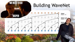

Andrej Karpathy: Tesla AI, Self-Driving, Optimus, Aliens, and AGI | Lex Fridman Podcast #333