CS231n Winter 2016: Lecture 11: ConvNets in practice
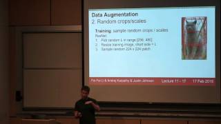
In this lecture Andrej Karpathy walks through the practical aspects of training convolutional neural networks (CNNs). After brief administrative announcements, he introduces three major themes: (1) data augmentation and transfer learning for small datasets, (2) designing and stacking convolutional layers efficiently, and (3) low‑level implementation details that affect speed and memory. He explains how simple augmentations (flipping, random crops, color jittering, PCA‑based color perturbation) act as stochastic regularizers and how they are applied at test time via multi‑crop averaging. He then covers transfer learning strategies—using pretrained ImageNet models as fixed feature extractors, fine‑tuning varying numbers of top layers, and practical tips such as learning‑rate schedules for frozen, newly‑initialized, and fine‑tuned layers. The lecture dives deep into convolution design: receptive‑field growth, why stacking 3×3 filters approximates larger filters, parameter and compute savings of 3×3 stacks versus a single 7×7, the 1×1 bottleneck sandwich (reduce‑compute, increase non‑linearity), factorising 3×3 into 3×1 and 1×3, and how these ideas appear in VGG, GoogLeNet, and ResNet. Implementation techniques are surveyed: im2col → matrix multiplication, FFT‑based convolution (useful only for large kernels), Strassen‑like fast algorithms for 3×3, and the importance of cuDNN/cuBLAS. He discusses hardware considerations: CPU vs GPU parallelism, data‑parallel multi‑GPU training (synchronous vs asynchronous SGD), model‑parallel tricks, and the role of TensorFlow and other frameworks. Finally, he highlights common bottlenecks (CPU‑GPU memory transfer, disk I/O, GPU memory limits) and the impact of numeric precision, from 32‑bit to 16‑bit half‑precision, stochastic rounding for low‑bit fixed‑point, and recent binary‑weight networks. The lecture ends with a recap of the four practical takeaways.
Chapters
All right. So I— we have a lot of stuff to get through today. So I'd like to get started. So today we're going to talk about CNNs in practice and talk about a lot of really low-level sort of implementation details that are really common to get these things to work, um, when you're actually training things. Uh, but first as usual we have some administrative stuff to talk about. Um, number one is that through a really heroic effort by all the TAs, all the midterms are already graded. So I— you guys should definitely thank them for that. And you can either pick them up after class today or in any of these office hours that are up here. Also, keep in mind that your project milestones are going to be due tonight at midnight. So make sure that— I hope you've been working on your projects for the last couple— for the last week or so and have made some really exciting progress. So make sure to write that up and put it in the assignments tab on Dropbox. No, no, not on Dropbox. Put it on the Assignments tab on Coursework. Sorry, I know this has been really confusing, but Assignments tab, just like Assignment 2. Assignment 2, we're working on grading. Hopefully we'll have that done sometime this week-ish. And remember that Assignment 3 is out. So how's that been going? Anyone done? OK, that's good. One person's done. So the rest of you should get started because it's due in a week. So we have some fun stats from the midterm. So don't freak out when you see your grade, because we actually had this really nice, beautiful Gaussian distribution with a beautiful standard deviation. We don't need to batch normalize this thing. It's already perfect. I'd also like to point out that someone got a max score of 103, which means they got everything right and the bonus. So that means it wasn't hard enough, maybe. [SPEAKING CHINESE] We also have some per-question stats, like per-question breakdown on average score per every single question. Question in the midterm. So if you got something wrong and you want to see if everyone else got it wrong too, you can go check on these stats later on your own time. But we have stats for the true/false and the multiple choice. Keep in mind— so actually for 2 of the true/false, we decided during grading that they were a little bit unfair. We threw it out and just gave you all the points, which is why 2 of those are at 100%. We have these stats for all the individual questions. So go ahead and have fun with those later. Um, let's— so last time, I know it's been a while, but we had a midterm and we had, um, a holiday. But if you can remember, like, over a week ago, we were talking about recurrent networks. So we talked about how recurrent networks can be used for modeling sequences. You know, normally with these feedforward networks, um, they take an— they model this feedforward function. But these recurrent networks, we talked about how they can model, um, different kinds of sequence problems. We talked about two particular implementations of recurrent networks, um, vanilla RNNs and LSTMs. And you'll implement both of those on the assignment, so you should know what they are. Uh, we talked about how these, uh, recurrent net— recurrent neural networks can be used for language models, and, um, had some fun showing some sample generated text on— what is this? Shakespeare and algebraic geometry. So that's fun. Uh, we talked about how we can combine recurrent networks with convolutional networks to do image captioning. And we played a little bit this game of being, uh, RNN neuroscientists and diving into the cells of the RNNs and trying to interpret what they're doing. And we saw that sometimes we have these interpretable cells that are, for example, activating inside if statements, which is pretty cool. But today we're going to talk about something completely different. There are 3— we're going to talk about really a lot of low-level things that you need to know to get CNNs working in practice. So there's 3 major themes. It's a little bit of a potpourri, but we're going to try to tie it together. So the first is really squeezing all the juice that you can out of your data. So I know a lot of you, especially for your projects, you don't have large datasets. So we're gonna talk about data augmentation and transfer learning, which are two really powerful, useful techniques, especially when you're working with small datasets. Uh, we're gonna really dive deep into convolutions and, uh, talk a lot more about those, both, um, how you can design efficient architectures using convolutions and also how convolutions are efficiently implemented in practice. And then finally, we're gonna talk about something that usually gets lumped under implementation details and doesn't even make it into papers, But that's stuff like, uh, what is a CPU, what is a GPU, um, what kind of bottlenecks do you experience in training, how might you distribute training, uh, over multiple, over multiple devices. So that's a lot of stuff. Um, we should get started. So first, let's talk about data augmentation. Um, I think we've sort of mentioned this maybe in passing so far in the lectures but never really talked formally about it. So normally when you're training CNNs, you're really familiar with this type of pipeline. During training, you're going to load images and labels up off the disk. You're going to pipe the image through to your CNN. Then you're going to use the image together with the label to compute some loss function, then backpropagate and update the CNN and repeat forever. So that— you should be really familiar with that by now. The thing about data augmentation is we just add one little step to this pipeline, which is here. So after we load the image up off disk, we're going to transform it in some way. Before passing it to the CNN. And this transformation should preserve the label. So we're gonna compute loss, backpropagate, and update the CNN. So it's really simple. And the trick is just what kinds of transforms you should be using. Right. So data augmentation, the idea is really simple. It's sort of this way that lets you artificially expand your training set through clever usage of different kinds of transformations. So if you remember, the computer is really seeing these images as these giant grids of pixels. And there are these different kinds of transformations we can make that should preserve the label, but which will change all of the pixels. If you imagine like shifting that cat 1 pixel to the left, it's still a cat, but all the pixels are going to change. So that— so when you talk about data augmentation, you're sort of imagine that you're expanding your training set. These training exam— these new fake training examples will be correlated, but it'll still help you train models with, with bigger models with less overfitting. And this is very, very widely used in practice. Pretty much any CNN you see that's winning competitions or doing well on benchmarks is using some form of data augmentation. So the easiest form of data augmentation is horizontal flipping. If we take this cat and we look at the mirror image, the mirror image should still be a cat. And this is really, really easy to implement. In NumPy, you can just do it with a single call, a single line of code. Similarly easy in Torch, other frameworks. This is really easy, very widely used. Something else that's very widely used is to take random crops from the training images. So at training time, we're going to load up our image and we're going to take a patch of that image at a random scale and location, resize it to our fixed, uh, whatever size our CNN is expecting, and then use that as our training example. And again, this is very, very widely used. Just to give you a flavor of, um, how exactly this is used, I, I looked up the details for ResNet. So they actually at training time, each training image, they resize— they first pick a random number, resize the whole image so that the shorter side is that number, then sample a random 224 by 224 crop from the resized image, and then use that as their training example. So that's pretty easy to implement and usually helps quite a bit. So, uh, when you're using this form of data augmentation, usually things change a little bit at test time. So at training time, when you're using this form of data augmentation, the network is not really trained on full images. It's trained on these crops. So it doesn't really make sense or seem fair to try to force the network to look at whole images at test time. So usually in practice, when you're doing this kind of, uh, random cropping for data augmentation, at test time, you'll have some fixed set of crops and use these for testing. So very commonly, you'll see that— you'll see 10 crops. You'll take the upper left-hand corner, the upper right-hand corner, the two bottom corners and the center, that gives you 5, together with their horizontal flips gives you 10. So you'll take those 10 crops at test time, pass them through the network, and average the scores of those 10 crops. Um, so ResNet actually takes this a little bit one step further, and they actually do multi-scale— multiple scales at test time as well. Um, so this is something that tends to help performance in practice, and again, very easy to implement, very widely used. Another thing that we usually do for data augmentation is color jittering. So if you take this picture of a cat, maybe, maybe it was a little bit cloudier that day or a little bit sunnier that day. And if we would have taken a picture, then a lot of the colors would have been quite different. So one thing that's very common to do is just change the color a little bit of our training images before we feed it to the CNN. So a very simple way is just to change the contrast. This is again very easy to implement, very simple to do. Um, but actually in practice you'll see that this, uh, contrast jittering is a little bit less common. And what instead you see is this slightly more complex pipeline, um, using principal component analysis over all the pixels of the training data. Um, so the idea is that we— for each pixel in the training data is this vector of length 3, an RGB. And if we collect those pixels over the entire training dataset, you get a sense of what kinds of colors generally exist in the training data. Then using principal component analysis gives us 3 principal component directions in color space that kind of tell us what are the directions along which color tends to vary in the dataset. So then at test— at training time for color augmentation, we can actually use these principal components of the color of the training set to choose exactly how to jitter the, the color at training time. This is again a little bit more complicated, but it is pretty widely used. So this type of, uh, PCA-driven, uh, data augmentation for color, um, I think was introduced with the AlexNet paper in 2012, and it's also used in ResNet, for example. Um, so data augmentation is, is really this very general thing, right? You just want to think about for your dataset, what kinds of transformations do you want your classifier to be invariant to? And then you want to introduce those types of, uh, variations to your training data at training time. And you can really go crazy here and get creative and really think about your data and what types of invariances make sense for your data. So you, you might want to try like maybe random rotations, um, depending on your data, maybe rotations of a couple degrees make sense. You could try like different kinds of stretching and shearing to simulate maybe affine transformations of your data. Um, and you could really go crazy here and try to get creative and think of, um, interesting ways to augment your data. Another thing that I'd like to point out is this idea of data augmentation really fits into kind of a larger theme that now we've seen repeated many times throughout the course. And this theme, um, is that one way that's really useful in practice for preventing overfitting, uh, as a regularizer, is that during the forward pass during training when we're training our network, we add some kind of weird stochastic noise to kind of mess with the network. Um, For example, with data augmentation, we're actually modifying the training data that we put into the network. With things like dropout or DropConnect, you're, uh, taking random parts of the network and either setting the activations or the weights to 0 randomly. Um, th— this also has— this also appears kind of with batch normalization. Um, since with batch normalization, your normalization contents depend on the other things in the mini-batch. So your normal— and during training, the same image might end up appearing in mini-batches with different other images. So that actually introduces this type of noise at training time. But for— in all of these examples at test time, we average out this noise. So for data augmentation, we'll take averages over many different samples of the training data. Um, for dropout and DropConnect, you can sort of evaluate and marginalize this out, um, more analytically. Um, and for batch normalization, we keep, keep these running means. So I just think that's kind of a nice way to unify a lot of these ideas for regularization, is that when you can add noise at the forward pass and then marginalize over it at test time. So maybe keep that in mind if you're trying to come up with other creative ways to regularize your networks. So that's— so the main takeaways for data augmentation are that one, it's, it's usually really simple to implement. Um, so you should almost always be using it. There's not really any excuse not to. Um, it's very, very useful especially for small datasets which I think many of you are using for your projects. Um, and it also fits in nicely with this framework of noise at training and marginalization at test time. So I think that's, that's pretty much all there is to say about data augmentation. So if there's any questions about that, I'm happy to talk about it now. Yeah. Do you typically pre-compute your augmented dataset or do you resample live as you're training? Yeah, that's a good question. So a lot of times you'll actually resample it live at training time, um, because it would take a lot of disk space to try to dump these things to disk. So a lot of time— so sometimes people get creative and even have like background threads that are fetching data and performing the augmentation. All right. So if I think that's— if that's clear, we can talk about the next idea. So there's this myth floating around that when you work with CNNs, you really need a lot of data. Um, but it turns out that with transfer learning, this myth is busted. So there's this really simple, uh, recipe that you can use for transfer learning. And that's first, you take whatever your favorite CNN architecture is, be it, uh, AlexNet or VGG or what have you, and you either train it on ImageNet yourself, or you down— or more commonly, you download a pre-trained model from the internet. That's easy to do, just takes a couple minutes to download, many hours to train, but you probably won't do that part. Next, um, there are sort of two general cases. One, if your dataset is really small and you really don't have any images whatsoever, then you can just treat this classifier as a fixed feature extractor. So one way to look at this is that you'll take the last layer of the network, um, the softmax, you— if it's an ImageNet classification model, you'll take it away and you'll replace it with some kind of linear classifier for the task that you actually care about. And now you'll freeze the rest of the network and retrain only that top layer. Um, so this is sort of equivalent to just training a linear classifier directly on top of features extracted from the network. So what you'll see a lot of times in practice for this case, is that sort of as a preprocessing step, you'll just dump features to disk for all of your training images and then work entirely on top of those cached features. So that can help speed things up quite a bit. And, and that's quite easy to use. It's very, very common. And it usually provides a very strong baseline for a lot of problems that you might encounter in practice. And if you have a little bit more data, then, then you can actually afford to train more complex models. So depending on the size of your dataset, um, usually you'll freeze some parts, some of the lower layers of the network, and then instead of retraining only the last layer, you'll pick some number of the last layers to train depending on how large your dataset is. And generally when you have a larger dataset available for training, you can afford to train more of these final layers. Um, and again, if you're similar to the, similar to the trick over here, um, what you'll see very commonly is that instead of actually explicitly computing this part, you'll just dump these last layer features to disk and then work on this part in memory. So that can speed things up quite a lot. Um, and sometimes act— oh, yeah, question? What would you consider to be like a small or a medium-sized dataset? Um, that you, you basically have to try it and see, but especially for this type of small dataset, we'll work on instances. So if you have like, if you wanna just do image retrieval, a pretty strong baseline is just to use L2 distance on CNN features. So maybe— so this type of approach, I mean, however many, however many samples you expect to need to train a, like, an SVM or something. And for these, if you have more than— if you have more data than you would expect to need for an SVM, then try that. So that's a little hand-wavy, I'm sorry. Yeah? So you still need all the weights for each layer because you still, like, run, run it through the forward pass, you just don't do —backpropagation to update? It depends. Sometimes you actually will run through the forward pass, but sometimes you'll just run the forward pass once and dump these to disk. That's pretty common, actually, because then it saves compute. Yeah? Actually, going off that question, so when you're freezing a certain part of the network, does that then mean that retraining on the part that you actually care about just means you're propagating —part of the loss. Yeah. Yeah. So then, so then typically this, this final layer you'll always need to swap in and reinitialize from random because you'll probably have different classes or you'll do— you're doing a regression problem or something. But then these, these other intermediate layers you'll initialize from whatever was in the pre-trained model. Um, and actually in, in practice when you're fine-tuning, um, uh, a nice tip to, to actually do this is that there'll, there'll really be two types of layers when you— well, I guess three types of layers when you're fine-tuning. Um, there'll be the frozen layers which you can think of as having a learning rate of 0. There are these, um, these new layers that you've re-initialized from scratch. And typically those have maybe a higher learning rate but not too high, maybe 1/10 of what the network was originally trained with. And then you'll have these intermediate layers that you are initializing from the pre-trained network, but you're planning to modify during optimization and fine-tuning. So these intermediate layers, you'll tend to have a very small learning rate, maybe 1/100th of the original. Um, yeah. Will this only work if, if your task is roughly similar to what the, the lower levels were trained for? Uh, that's a, that's a good question. Some people have tried to investigate that and found that, um, generally fine-tuning this type of transfer learning fine-tuning approach works better when the network was originally trained with similar types of data, whatever that means. But in fact, these, these very low-level features are things like edges and colors and Gabor filters, which are probably going to be applicable to just about any type of visual data. So especially these lower-level features, I think, are generally pretty applicable to almost anything. And by the way, another tip that you, that you sometimes see in practice for fine-tuning is that you might actually have a multi-stage approach where first you freeze the entire network, and then only train this last layer. And then after this last layer seems to be converging, then go back and actually fine-tune these. Um, you can sometimes have this problem that, um, these— because this last layer is initialized randomly, you might have very large gradients that kind of mess up this initialization. So the, the two ways that we get around that are either freezing this at first and letting this converge, or by having this varying learning rate between the two regimes of the network. Um, so this idea of transfer learning actually works really well. So there was a couple, uh, pretty early papers from 2013, 2014 when CNNs first started getting popular. Um, this one in particular, the astounding baseline paper, was, was pretty cool. What they did is they took the, what at the time was one of the best CNNs out there was Overfeat. So they just extracted features from Overfeat, and applied these features to a bunch of different standard datasets and standard problems in computer vision. And they compared these, um, right, so then the idea is that they compared against what was at the time these very specialized pipelines and very specialized architectures for each individual problem and dataset. And for each problem, they just replaced this very specialized pipeline with very simple linear models on top of, uh, features from OverFeat. And they did this for a whole bunch of different datasets. And found that in general overall these overfit features were a very, very strong baseline. Um, and for some problems they were actually better than the existing methods, and for some problems they were a little bit worse but still quite competitive. So this, this was I think a really cool paper that just demonstrated that these are really strong features that can be used in a lot of different tasks and tend to work quite well. Um, another paper along those lines was from Berkeley, uh, the decaf paper. Um, and decaf later became became caffeinated and became café. So that's, that's, that's kind of the lineage there. Um, so kind of the recipe for transfer learning is that there— you should kind of think about two— this little 2x2 matrix. Um, how similar is your dataset to what the pre-trained model was, and how much data do you have, and what should you do in those four different columns? So generally, if you have a very similar dataset and very little data, just using, uh, the network as a fixed feature extractor, and training simple, maybe linear models on top of those features tends to work very well. Um, if you have a little bit more data, then you can try, try fine-tuning and try actually initializing the network from fine-tune— from pre-trained weights and running optimization from there. Um, this other column is a little trickier. In this box, you might be in trouble. Um, you can try to get creative and maybe instead of extracting features from the very last layer, you might try extracting features from different layers of the ConvNet. And that can sometimes, sometimes help. Um, the intuition there is that maybe for something like MRI data, probably these very top-level features are very specific to ImageNet categories, but these very low-level features are things like edges and, and stuff like that, that may be more transferable to, um, to non-image— to non-ImageNet type datasets. And obviously in this box, you're in better shape. And again, you can just sort of initialize and fine-tune. So another thing I'd like to point out is this idea of, um, initializing with pre-trained models and fine-tuning is actually not the exception. This is pretty much standard practice in almost any larger system that you'll see in computer vision these days. And we've actually seen two examples of this already in the course. So for example, if you remember from a few lectures ago, we talked about object detection where we had a CNN looking at the image and region proposals and this other, all this, all this crazy stuff, but this part was a CNN looking at the image. And for image captioning, we had a CNN looking at the image. So in both of those cases, those CNNs were initialized from ImageNet models. And that really helps, um, to solve these other more specialized problems even without gigantic datasets. And also for the image captioning model in particular, part of this model includes these word embeddings that you should have seen by now on the homework if you started on it. Um, but those word vectors you can actually initialize from something else that was maybe pre-trained on a bunch of text. And that can sometimes help maybe in some situations where you might not have a lot of captioning data available. Yeah? [Speaker:AUDIENCE] On the previous slide, has anybody tried collecting features from multiple layers and concatenating them? [Speaker:ANDREJ KARPATHY] So that was like on here or maybe here? Yeah, yeah, people have definitely tried that. And that tends to help sometimes. It depends on the problem, depends on the network, but it's definitely something you can try. And that especially might help when you're in this box. But yeah, that's a good trick. All right. So the takeaway about fine-tuning is that, um, you should really use it. It's a really good idea. Um, yeah. So that it works really well in practice. You should probably almost always be using it to some extent. Um, you generally don't want to be training these things from scratch unless you have really, really large datasets available. In almost all of the circumstances, it's much more convenient to fine-tune an existing model. Um, and by the way, Caffe has this existing model view. You can download many, um, exist— many, uh, famous ImageNet models. Um, uh, actually the residual networks, the official model got released recently, so you can even download that and play with it. That'd be pretty cool. Um, and these Caffe Model Zoo models are sort of like a, a little bit of a standard in the community. So you can even load Caffe models into other frameworks like Torch. So that's something to keep in mind, that these Caffe models are quite useful. All right. Any further questions on fine-tuning or transfer learning? Yeah? Yeah, I just have a question. So you're talking about like for different types of images, you might wanna pull lower-level layers instead of like the FC 4096 layer or whatever. Isn't it true that at lower levels you just have like a huge, huge number of features? Yeah, that's true. 3-dimensional box. Yeah. So that's, that's true. The feature dimension is quite large at lower dimensions. So you might try a highly regularized linear model on top of that, or you might try putting a small ConvNet on top of that to maybe reduce the dimensionality. You can get creative here, but I think that there are, there are, there are things you can try that might work for your data depending on it. All right, so I think we should talk more about convolutions. So for, for all these networks we've talked about, really the convolutions are the computational workhorse that's doing a lot of the work in the network. So we need to talk about two things about convolutions. The first is how to stack them. So how can we design efficient network architectures that combine many layers of convolution to achieve some, some nice results? So here's a question. Suppose that we have a network that has 2 layers of 3x3 convolutions. So this would be the input. This would be the activation map in the first layer. This would be the activation map after 2 layers of convolution. So the question is, for a neuron on this second layer, how big of a region on the input does it see? This was on your midterm, so I hope, I hope you guys all know the answer to this. Murmurs? Anyone? OK. I guess maybe that was a hard midterm question. But this is a 5 by 5. And it's pretty easy to see from this diagram why. So that this neuron after the second layer is looking at this entire volume in the intermediate layer. So in particular, this pixel in the intermediate layer is looking at this 3 by 3 region in the input. So when you average across— when you look at all of— all 3 of these, then this layer— this neuron in the third layer is actually looking at this entire 5 by 5 volume in the input. OK. So now the question is, if we had 3 3 by 3 convolutions stacked in a row, how big of a region in the input would they see? [Speaker:AUDIENCE] Same width. [Speaker:ANDREJ KARPATHY] Yeah, good. So same kind of reason, that these receptive fields just kind of build up with successive convolutions. Um, so the point here to make is that, you know, 3 3x3 convolutions actually give you a very similar representational power, um, is my claim, to a single 7x7 convolution. So it— you, you might debate on the exact semantics of this and you could try to prove theorems about it and things like that. But just from an intuitive sense, they can— 3 3x3 convolutions can represent similar types of functions as a similar 7x7 convolution. Since it's looking at the same input region, um, in the input. So now the ide— now actually we can dig further into this idea and we can compare more concretely between, um, a single 7x7 convolution versus a stack of 3, 3x3 convolutions. So let's suppose that we have an input image that's H by W by C, um, and we want to have convolutions that preserve the depth. So we have C filters, and we want to have them preserve height and width. So we just set padding appropriately. And then we want to compare concretely, um, what is the difference between a single 7x7 versus a stack of 3x3. So first, um, how many weights do each of these two things have? Anyone have a guess on how many weights the, the single 7x7 convolution has? Uh, you can forget about biases because they're confusing. Uh, I heard, I heard some, some murmurs, but so my, my answer, I hope I got it right, was 49C squared because you've got this 7 by 7 convolution. Each one is looking at a depth of C, and you've got C such filters, so 49C squared. Um, but now for the 3 by 3 convolutions, we have 3 layers of convolutions. Each one— each filter is 3 by 3 by C, and each layer has C filters. When you multiply that all out, we see that 3 3 by 3 convolutions only has 27 C squared parameters. And assuming that we have ReLUs after between each of these convolutions, we see that the stack of 3 3 by 3 convolutions actually has fewer parameters, which is good, and more nonlinearity, which is good. So this kind of gives you some intuition for why a stack of 3 by— of multiple 3 by 3 convolutions might actually be preferable to a single 7 by 7 convolution. And we can actually take this one step further and think about not just the number of learnable parameters, but actually how many floating point operations do these things take. So anyone have a guess for how many, how many operations these, these two take? Guess not? Sounds hard? Right. So actually this is pretty easy because for each of these filters, we're going to be using it at every position in the image. So actually the number of multiply adds is just going to be height times width times the number of learnable filters. So you can see that actually over here, again, not only do we have— so between— like comparing between these two, the 7x7 actually not only has more learnable parameters, but it actually costs a lot more to compute as well. So the stack of, of 3 3x3 convolutions again gives us more nonlinearity for less compute. So that kind of gives you some intuition for why actually having multiple layers of 3x3 convolutions is actually preferable to large filters. Um, but then you can think of another question. You know, we've been pushing towards smaller and smaller filters, But why stop at 3 by 3, right? We can actually go smaller than that. Maybe the same logic would extend. You're shaking your head, you don't believe it? [Speaker:AUDIENCE] You don't get the receptive field. [Speaker:ANDREJ KARPATHY] That's true. That's true. You don't get the receptive field. So actually what we're going to do here is compare a single 3 by 3 convolution versus a slightly fancier architecture called a bottleneck architecture. So here we're going to assume, again, an input of HWC. And here we can actually do— this is a cool trick. We do a single 1x1 convolution with C/2 filters to actually reduce the dimensionality of the volume. So now this thing is going to have the same spatial extent but half the number of features in depth. Now after we do this bottleneck, we're going to do a 3x3 convolution at this reduced dimensionality. So now this 3x3 convolution takes C/2 input features and produces C/2 output features. And now we restore the dimensionality with another 1 by 1 convolution to go from C over 2 back to C. So this is kind of a, kind of a funky architecture. This idea of using 1 by 1 convolutions everywhere is sometimes called network in network because it has this intuition that your 1 by 1 convolution is kind of similar to sliding a fully connected network over each part of your, of your input volume. And this idea also appears in GoogLeNet and in ResNet, this idea of using these 1x1 bottleneck convolutions. So we can compare this bottleneck sandwich to a single 3x3 convolution with C filters and run through the same logic. So I won't, I won't force you to compute this in your heads, but you'll have to trust me on this, that this bottleneck stack has 3.25 C squared parameters, whereas this one over here has 9 C squared parameters. And again, if we're sticking ReLUs in between each of these convolutions, then this bottleneck sandwich is giving us more, more nonlinearity for a fewer number of parameters. And actually, so we— as we— similar to we saw on the, on the 3 by 3 versus 7 by 7, the number of parameters is tied directly to the amount of computation. So this bottleneck sandwich is also much faster to compute. So this, this idea of 1x1 bottlenecks has received quite a lot of usage recently in GoogleNet and ResNet especially. Yeah? What's the point of the last 1x1? Like you have these columns of C/2 and you're just smearing the same information over? Well, those, those convolutions are learned. So you might think of it as, sometimes you think of it as, uh, as a projection from like a lower dimensional feature back to a higher dimensional space. And then if you think about stacking many of these things on top of each other as happens in ResNet, then, then you— then coming immediately after this one is going to be another 1 by 1. So you're kind of stacking many, many one— multiple 1 by 1 convolutions on top of each other. And a 1 by 1 convolution is a little bit like sliding a fully— a multi-layer fully connected network over each depth channel. You'll have to think— maybe think about that one a little bit. But it turns out that actually you don't really need the spatial extent. And even just comparing this sandwich to a single 3x3 conv, you're sort of having the same input-output volume sizes, but with more non-linearity and cheaper to compute and fewer learnable parameters. So those are all kind of nice features. But there's, there's one problem with this is that, and that's we're still using a 3x3 convolution in there somewhere. And you might wonder if we, if we really need this. And the answer is no, it turns out. So, One crazy thing that I've seen recently is that you, you can factor this 3x3 convolution into a 3x1 and a 1x3. And compared with a single 3x3 convolution, this ends up saving you some parameters as well. So then you might, you, if you really go crazy, you can combine this 1x3 and 3x1 together with this bottlenecking idea and, and things just get really cheap. And that's basically what Google has done in their most recent version of Inception. So there's this kind of crazy paper, um, Rethinking the Inception Architecture for Computer Vision, where they play a lot of these crazy tricks about factoring convolutions in weird ways and having a lot of 1x1 bottlenecks and then projections back up to different dimensions. And if you thought the original GoogleNet with, with their inception module was, was crazy, um, this one's— these are the inception modules that Google is now using in their newest inception net. And the interesting features here are that they have these 1x1 bottlenecks everywhere, and actually you have these asymmetric filters to again save on computation. So this stuff is not super widely used yet, but it's, it's, it's out there and it's in GoogleNet. So I thought it's, it's something cool to mention. So the, the quick recap from convolutions and, and how to stack them is that it's usually better instead of having a single large convolution with a large filter size, it's usually better to break that up into multiple smaller filters. And that even maybe helps explain the difference between something like VGG, which has many, many 3x3 filters, with something like AlexNet that had fewer smaller filters. Um, some— another thing that's actually become pretty common, I think, is this idea of 1x1 bottlenecking. You see that in, in both versions of GoogleNet and also in ResNet. And that actually helps you save a lot on parameters. So I think that's a useful trick to keep in mind. And this idea of factoring convolutions into these asymmetric filters, I think, is maybe not so widely used right now, but it may become more commonly used in the future. I'm not sure. And the, the basic overall overarching theme for all of these tricks is that it lets you have fewer learnable parameters, and few— and less compute, and more non-linearity, which are all sort of nice features to have in your architectures. So if there's any questions about these convolution architecture designs? Too boring or too obvious? [LAUGHTER] OK, so then the next thing is that once you've actually decided on how you want to wire up your stack of convolutions, you actually need to compute them. And this— there's actually been a lot of work on different ways to implement convolutions. We asked you to implement it on the assignments using for loops, and that, as you may have guessed, doesn't scale too well. So this— a pretty easy approach that's pretty easy to implement is this idea of an im2call method. So the intuition here is that we know matrix multiplication is really fast. And pretty much for any computing architecture out there, someone has written a really, really well optimized matrix multiplication routine or library. So the idea of im2call is thinking, well, given that matrix multiplication is really fast, is there some way that we can take this convolution operation and recast it as a matrix multiply? And it turns out that this is actually pretty, uh, somewhat easy to do once you think about it. So the idea is that, um, we have an input volume that's H by W by C, and we have a filter bank of convolutions, uh, of convolutional filters. Each one of these is going to be a K by K by C volume. So it has a K by K receptive field and a depth of C. To match the, to match the input over here. And we're going to have d of these filters. And then we want to turn this into a matrix multiply problem. So the idea is that we're going to take one of the— we're going to take the first receptive field of the image, which is going to be this k by k by c region in the input region— in the input volume. And we're going to reshape it into this column of k squared by c elements. And then we're going to repeat this for every possible receptive field in the image. So we're going to take this little guy, and we're going to shift him over all possible regions in the image. And here I'm just saying that there's going to be maybe n region— n different receptive field locations. So now we've taken our image, and we've reshaped it into this giant matrix of n by— I mean, n by k squared by c. Anyone see what a potential problem with this might be? Yeah? [Speaker:AUDIENCE] You may have a lot more [Speaker:ANDREJ KARPATHY] Yeah, that's true. So this tends to use a lot of memory, right? So any elements in this input volume, if it appears in multiple receptive fields, then it's going to be duplicated in multiple of these columns. And this is going to get worse the more overlap there is between your receptive fields. But it turns out that in practice, that's actually not too big of a deal, and it works fine. So then we're going to run a similar trick on these convolutional filters. So if you remember what a convolution is doing, we want to take each of these convolutional weights and take inner products with each convolutional weight against each receptive field location in the image. So each of these convolutional weights is, is this K by K by C tensor. So we're going to reshape each of those to be a K squared by C row. And now we have D filters, so we get a D by K squared by C matrix. So now this is great. Um, now this guy contains all the recep— each, each column is a receptive field, and we have one column per receptive field in the image. And now this matrix has one, uh, has one— each row is a different weight. So now we can easily compute, uh, all of these inner products all at once with a single matrix multiply. And this— I apologize for these dimensions not working out. I probably should have swapped these two to make it more obvious, but I think you get the idea. So this gives you a D by N result. So that D is our number of output filters, and that N is for all the receptive field locations in the image. So then you play a similar trick to take this and reshape it into your 3D output tensor. And you can actually extend this to mini-batches quite easily. If you have a mini-batch of n of these elements, you just add more rows and have 1 set of rows per mini-batch element. So this actually is pretty easy to implement. So a lot— oh, yeah, question? [Speaker:AUDIENCE] How expensive is the reshape operation? [Speaker:ANDREJ KARPATHY] It depends. That's then— it depends on your implementation, right? But then you have to worry about things like memory layout and stuff like that to make it fast. But sometimes you'll even do that reshape operation on the GPU so you can do it in parallel. But as a case study— so this is really easy to implement. So a lot of— if you don't have a convolution technique available and you need to implement one fast, this is probably the one to choose. And if you look at actually Caffe, in early versions of Caffe, this is the method that they use for doing convolutions. So this is the convolution forward code. For the GPU— like the native GPU convolution in Caffe. So you can see in this red chunk, they're calling into this im2col method that's taking their input image. Right? So this is taking their input image somewhere. This is— right? So this is their input image. And then they're going to reshape this calling this im2col method and then store it in this column GPU tensor. Then they're going to take— do a matrix multiply, calling into cuBLAS to do the matrix multiply, and then add the bias. So that's how— I mean, these things tend to work quite well in practice. And also as another case study, if you remember the fast layers we gave you in the assignments, actually uses this exact same strategy. So here we actually do an im2col operation with some crazy NumPy tricks. And then now we can actually do the convolution inside the fast layers with a single call to the NumPy matrix multiplication. And you saw in your homeworks this usually gives maybe a couple hundred times faster than using for loops. So this actually works pretty well and it's pretty easy to implement. Any questions about im2col? Yeah? [Speaker:AUDIENCE] How does that work in reverse? [Speaker:ANDREJ KARPATHY] Yes, then you have to think about it a little bit. But if you think really hard, you'll realize that the backward pass on a convolution is actually also a convolution. Which you may have figured out if you were thinking about it on your homework. But the backward pass of a convolution is actually also a type of convolution over the upstream gradients. So you can actually use a similar type of im2call method for the backward pass as well. The only trick there is that once you do— in the backward pass, you need to sum gradients from across overlapping receptive fields in the upstream. So you need to be careful about the call to im you need to sum in the call to im in the backward pass. And you can actually check out in the fast layers in the homework, it implements that too. Although actually for the— in the fast layers in the homework, the call to im is in Cython. I couldn't find a way to get it fast enough in raw NumPy. So there's actually another way that sometimes people use for convolutions. And that's this idea of a fast Fourier transform. So if you have some memories from like a signal processing class or something like that, you might remember this thing called the convolution theorem. And that says that if you have two signals and you want to convolve them either discretely or continuously with an integral, then taking a convolution of these two signals is the same as— rather, the Fourier transform of the convolutions is the same as the element-wise product of the Fourier transforms. So if you unpack that and stare at the symbols, I think it'll make sense. And if also you might remember from, again, a signal processing class or an algorithms class, that there's this amazing thing called the fast Fourier transform that actually lets us compute Fourier transforms and inverse Fourier transforms really, really fast. You may have seen it. There's versions of this in 1D and 2D, and they're all really fast. So we can actually apply this trick to convolutions. So the way that this works is that first we're going to compute— use the fast Fourier transform to compute the Fourier transform of the weights, um, also compute the Fourier transform of our activation map. And now in Fourier space, we just do an element-wise, uh, multiplication, which is really, really fast and efficient. And, um, then we just com— again use, uh, the fast Fourier transform to do the inverse transform on the output of that element-wise product. And that implements convolutions for us in this kind of cool, fancy, clever way. And this has actually been used. And face— some folks at Facebook had a paper about this last year. And they actually released a GPU library to do this, to compute these things. But the sad thing about these Fourier transforms is that they actually give you really, really big speedups over other methods, but really only for large filters. And when you're working on these small 3 by 3 filters, the overhead of computing the Fourier transform just dwarfs the computation of doing the computation directly in the input pixel space. And as we just talked about earlier in the lecture, those small convolutions are really, really nice and appealing and great for lots of reasons. So it's a little bit of a shame that this Fourier trick doesn't work out too well in practice. But if for some reason you do want to compute really large convolutions, then this is something you can try. Yeah? [Speaker:AUDIENCE] Yeah, so when you're doing that, is there an issue with spectral resolution on Fourier transforms? So in the sense that if I was going to do this normally in single processing, I would maybe do a convolution. I'd have a Hamming window on the convolution before I get it back. Is that something that matters? Do we care about it? Or is that something you can use as additional parameters? [Speaker:ANDREJ KARPATHY] I'm not entirely sure. I'm actually not too involved in Fourier stuff. But I imagine if you think it's a problem, it's probably a problem. Yeah, although another thing to point out is that one kind of downside about Fourier transforms convolutions is that they don't handle striding too well. So for normal compute— when you're computing strided convolutions in sort of normal input space, you only compute a small subset of those inner products. So you actually save a lot of computation when you do strided convolutions directly on the input space. But the way you tend to implement strided convolutions in Fourier transform space is you just compute the whole thing and then you throw out part of the data. So that ends up not being very efficient. So there's another trick that has not really become too, I think, too widely known yet, but I really like it, so I thought I wanted to talk about it. So you may remember from an algorithms class something called Strassen's algorithm, right? So there's this idea that when you do a naive matrix multiplication of two n by n matrices, kind of if you count up all the multiplications and additions that you need to do, it's going to take about— it's going to take n cubed operations. And Strassen's algorithm is this like really crazy thing where you compute all these crazy intermediates and it somehow magically works out to compute the output asymptotically faster than the naive method. And you know, from Imtacol, we know that matrix multiplication is this— we can implement convolution as matrix multiplication. So intuitively, you might expect that these similar types of tricks might theoretically maybe be applicable to convolution. And it turns out they are. So there's this really cool paper that just came out over the summer where these two guys worked out very explicitly some very special cases for 3x3 convolutions. And it involves this— obviously, I'm not going to go into details here, but it's a similar flavor to Strassen's algorithm. Where you're computing very clever intermediates and then recombining them to actually save a lot on the computation. And these guys are actually really, really intense, and they are not just mathematicians. They actually wrote also highly, highly optimized CUDA kernels to compute these things and were able to speed up VGG by a factor of 2. So that's really, really impressive. So I think that these type— this type of trick might become pretty popular in the future. But for the time being, I think it's not very widely used. But these numbers are crazy. And especially for small batch sizes, they're getting a 6x speedup on VGG. So that's, that's really, really impressive. And I think it's a really cool method. The downside is that you kind of have to work out these explicit special cases for each different size of convolution. But maybe if we only care about 3x3 convolutions, that's not such a big deal. So the recap on computing convolutions in practice. Is that the really fast, easy, quick and dirty way to implement these things is im2call. Matrix multiplication is fast. It's usually not too hard to implement these things. So if for some reason you really need to implement convolutions yourself, I'd really recommend im2call. FFT is something that coming from signal processing you might think would be really cool and really useful. But it turns out that it does give speedups, but only only for big filters, so it's not as useful as you might have hoped. But there is hope because these fast algorithms are really good at small filters, and there already exists code somewhere in the world to do it. So hopefully these things will catch on and become more widely used. So if there's any questions about computing convolutions? No? OK. Next we're going to talk about some implementation details. First I have a question. How many of you guys have ever built your own computer? Some? Okay. You guys are prevented from answering on this next slide. Who can spot the CPU? Anyone want to point it out? [Speaker:AUDIENCE] [INAUDIBLE] Yeah, so the CPU is this little guy. So actually, this thing is actually— a lot of it is the cooler. So the CPU itself is a little tiny part inside of here. A lot of this is actually the heat sink and the cooling. So next, who can spot the GPU? [LAUGHTER] Yeah, it's the thing that says GeForce on it. So this GPU is, for one thing, it's much larger than the CPU. So it maybe is more powerful. I don't know. But at least it's taking up more space in the case. So that's kind of an indication that something exciting is happening. So I have another question. Any of you guys play video games? OK. Then you probably have opinions about this. So it turns out a lot of people in machine learning and deep learning have really strong opinions too. And most people are on this side. So NVIDIA is actually much, much more widely used than AMD for using GPUs in practice. And the reason is that NVIDIA has really done a lot in the last couple of years to really dive into deep learning and make it a really core part of their focus. So as a cool example of that, um, last year at, uh, GTC, which is, uh, NVIDIA's, um, sort of yearly big gigantic conference where they announce new products, uh, Jensen Huang, who's the CEO of NVIDIA and actually also a Stanford alum, uh, introduced this latest and greatest amazing new GPU called the Titan X, like their flagship thing. And the benchmark he used to sell it was how fast it can train AlexNet. So this was crazy. This was a gigantic room with like hundreds and hundreds of people and journalists and like this gigantic highly polished presentation. And the CEO of NVIDIA was talking about AlexNet and convolutions. And I thought that was really exciting. And it kind of shows you that NVIDIA really cares a lot about getting these things to work. And they've pushed a lot of their efforts into getting things— into making it work. So just to give you an idea, a CPU, as you probably know, is really good at fast sequential processing, and they tend to have a small number of cores. Ones in your laptop probably have like maybe between 1 and 4 cores, and big things on a server might have up to 16 cores-ish. And these things are really good at computing things really, really fast and in sequence. GPUs, on the other hand, tend to have many, many, many cores. For a big guy like a Titan X, it can have up to thousands of cores. But they tend— each core can do less. They tend to run at a lower clock speed and be able to do less per instruction cycle. So these GPUs, again, were actually originally developed for processing graphics— graphics processing units. And so they're really good at doing sort of highly parallelized operations where you want to do many, many things in parallel independently. And since they were originally designed for computer graphics, but since then they've sort of evolved as a more general computing platform. So there are different frameworks that allow you to write generic code to run directly on the GPU. So from NVIDIA, we have this framework called CUDA that lets you write a variant of C to actually write code that runs directly on the GPU. And there's a similar framework called OpenCL that works on pretty much any computational platform. But I mean, open standards are nice, and it's quite nice that OpenCL works everywhere. But in practice, CUDA tends to be a lot more performant and have a little bit nicer library support. So at least for deep learning, most people use CUDA instead. And if you're interested in actually learning how to write GPU code yourself, there's a really cool Udacity course. I would— it's pretty cool. They have fun assignments, all that. That lets you write code to run things on a GPU. Although in practice, if all you want to do is train ConvNets and do research and that sort of thing, you end up usually not having to write any of this code yourself. You just rely on external libraries. Yeah? Is cuDNN kind of like Caffe and Torch, or what does it provide? Yeah, so cuDNN is— I'll talk about that in a minute. So cuDNN is a higher-level library, kind of like cuBLAS. So one thing that GPUs are really, really good at is matrix multiplication. So here's a benchmark. I mean, this is from NVIDIA's website, so it's a little bit biased. But this is showing matrix multiplication time as a function of matrix size on a pretty beefy CPU. This is a 12-core guy that would live in a server. So that's like quite a healthy CPU. And this is running the same size matrix multiply on a Tesla K40, which is a pretty beefy GPU. And it's much faster. I mean, that's no big surprise, right? And GPUs are also really good at convolutions. So as you mentioned, NVIDIA has a library called cuDNN that is specifically optimized— optimized CUDA kernels for convolution. So compared to CPU, I mean, it's way faster. And this is actually comparing the im2col convolutions from Caffe with the cuDNN convolutions. I think these graphs are actually from the first version of cuDNN. Version 4 just came out maybe a week ago. But this is the only version where they actually had a CPU benchmark. Since then, the benchmarks have only been against previous versions. So it's gotten a lot faster since then, since here. But the way this fits in is that something like cuBLAS or cuDNN is a C library. So it provides functions in C. That just sort of abstract away the GPU as a C library. So if you have a tensor sort of in, in memory in C, you can just pass a pointer to the cuDNN library, and it'll return the comp— it'll run it on the GPU maybe asynchronously and return the result. So frameworks like Caffe and Torch all have now integrated the cuDNN stuff into their own frameworks. So you can utilize these efficient convolutions in any of these frameworks now. Um, but the problem is that even when once we have these really powerful GPUs, training big models is still kind of slow. Um, so VGGNet was famously trained for something like 2 to 3 weeks on 4 Titan— what was it? Titan Blacks, and those aren't cheap. Um, and there was actually a reimplementation of ResNet recently. There's a really cool write-up, uh, there's a really cool blog post describing it here. And they actually retrained, uh, the ResNet 101-layer model, and it also took about 2 weeks to train on 4 GPUs. So that's not good. And one way that people— the way that— the easy way to split up training across multiple GPUs is just to split your mini-batch across the GPUs. So normally, you might have— you, especially for something like VGG, it takes a lot of memory. So you can't compute with very large mini-batch sizes on a single GPU. So what you'll do is you'll have a mini-batch of images, maybe of 128 or something like that. You'll split the mini-batch into 4 equal chunks on each, on each GPU. You'll compute a forward and a backward pass for that mini-batch. And you'll compute parameter gradients on the weights. You'll sum those weights inside, you'll sum those weights after all 4 GPUs finish and make an update to your model. So this is a really simple way that people tend to implement distribution on GPUs. Yeah? [Speaker:AUDIENCE] Just in theory, isn't this what TensorFlow is really good at? It's like automating across a bunch of GPUs. [Speaker:ANDREJ KARPATHY] Yeah, yeah. So one of the cool pitches of TensorFlow is they claim that they can automate this process and really, really efficiently distribute it, which is really exciting, I think. But I haven't played around with it too much myself yet. And also, at least in Torch, there's a data parallel layer that you can just drop in and use that will sort of automatically do this type of parallelism. Very easily. A slightly more complex idea for multi-GPU training actually comes from Alex Krizhevsky of AlexNet fame. He has— that's kind of a cool, kind of a funny title. But the idea— but the idea is that we want to actually do data parallelism on the lower layers. So on the lower layers, we'll take our image mini-batch, split it up across 2 GPUs, and GPU 1 will compute the convolutions for the first part, first part of the mini-batch, and just at least just this convolution part will be distributed equally across the GPUs. But once you get to the fully connected layers, he found it's actually more efficient if you— because those are just really big matrix multiplies, then it's more efficient to actually have the GPUs work together to compute this matrix multiply. So this is kind of a cool trick. It's not very commonly used, but I thought it's fun to mention. Another idea from Google is before, before there was TensorFlow, they had this thing called DistBelief, which was their previous system, which was entirely CPU-based, which from the benchmarks a few slides ago, you can imagine was going to be really slow. But actually the first version of GoogleNet was all trained in DistBelief on CPU. So they had to do massive amounts of distribution on CPU to get these things to train. So here, there's this cool paper from Jeff Dean a couple years ago that describes this in a lot more detail. But you use data parallelism, where you have each machine have an independent copy of the model. And you— each machine is computing forward and backward on batches of data. But now it actually— you actually have this parameter server that's storing the parameters of the model. And these independent workers are making communication with the parameter server to make updates on the model. And they contrast this with model parallelism, which is where you have one big model and you have different, different workers computing different parts of the model. So in, in disbelief, they really did a really good job optimizing this to work really well across many, many CPUs and many, many machines. But now they have TensorFlow, which hopefully should do these things more automatically. And once you're doing these updates, there's this idea between asynchronous SGD and synchronous SGD. So synchronous SGD is kind of the thing, like the naive thing you might expect. You have a mini batch, you split it up across multiple workers, each worker does forward and backward, computes gradients, then you add up all the gradients and make a single model update. This will, this will sort of exactly simulate just computing that mini batch on a larger machine. But it could be kind of slow since you have to synchronize across machines. This tends to not be too much of a big deal when you're working with multiple GPUs on a single node. But once you're distributing this across many, many CPUs, that, that synchronization can actually be quite expensive. So instead, at least, they also have this concept of asynchronous SGD where each model is just sort of making updates to the, to its own copy of the parameters. and those have some notion of eventual consistency where they sometimes periodically synchronize with each other. And it seems really complicated and hard to debug, but they got it to work. So that's, that's pretty cool. And one of the really cool pitches— so these two figures are both from the TensorFlow paper. And one of the pitches of TensorFlow is that it should really make this type of distribution much more transparent to the user. That if you do happen to have access to a big cluster of GPUs and CPUs and whatnot, TensorFlow should automatically be able to figure out the best way to do these kinds of distributions combining data and model parallelism and just do it all for you. So that's really cool. And I think that's the really exciting part about TensorFlow. Any questions about distributed training? Yeah. Do you have any thoughts on CNTK? On CNTK? I haven't taken a look at it yet. OK. So next, there's a couple bottlenecks you should be aware of in practice. So usually when you're training these things, this distributed stuff is nice and great, but you can actually go a long way with just a single GPU on a single machine. And there, there's a lot of bottlenecks that can get in the way. One is the communication between the CPU and the GPU. Actually, in a lot of cases, especially when the data is small, the most expensive part of the pipeline is copying the data onto the GPU and then copying it back. Once you get things onto the GPU, you can do computation really, really fast and efficiently. But the copying is the really slow part. So one idea is you want to make sure to avoid the memory copy. Like one thing that sometimes you see is like you'll— at each layer of the network is copying back and forth from CPU to GPU. And that'll be really inefficient and slow everything down. So ideally you want the whole forward and backward pass to run all on the GPU at once. Another thing you'll sometimes see is a multi-threaded approach where you'll have a CPU thread that is prefetching data off disk or off memory in one thread in the background. Possibly also applying data augmentations online. Um, and then this, this background CPU thread will be sort of preparing mini-batches and possibly also shipping them over to GPU. So you can kind of coordinate this loading of data and computing preprocessing and shipping memory— shipping the, uh, mini-batch data to the GPU and actually doing the computations. And actually you can get pretty involved with, um, coordinating all the— all these things in a multi-threaded way, and that can give you some good speedups. Café in particular I think already implements this prefetching data layer for certain types of data storages, and in other frameworks you just have to roll your own. Another problem is the CPU disk bottleneck. These things are kind of slow. They're cheap and they're big, but they actually are not the best. These are hard disks that— now these solid state drives are much more common. But the problem is that solid state drives are smaller and more expensive, but they're a lot faster, so they get used a lot in practice. So what's really— although one common feature to both hard disks and solid state drives is that they work best when you're reading data sequentially off the disk. So a lot of times what you'll— right, so one thing that would be really bad, for example, is to have a big folder full of JPEG images, because now each of these images could be located in different parts on the disk, so it could be really— you'd have to do a random seek to read any individual JPEG image. Image. And now also, once you read the JPEG, you'd have to decompress it into pixels, so that's quite inefficient. So what you'll see a lot of times in practice is that you'll actually preprocess your data by decompressing it and just writing out the raw pixels for your entire dataset in one giant contiguous file to disk. So that takes a lot of disk space, but we do it anyway because it's all for the good of the commonness. Right, so this is— so in Caffe, we do this with a couple— with like a LevelDB is one commonly used format. I've also used— I also use HDF5 files a lot for this. But the idea is that you want to just get your data all sequentially on disk and already turned into pixels. So then at training, when you're training, you can't store all your data in memory. You have to read it off disk. And you want to make that read as fast as possible. And again, with clever amounts of prefetching and multithreaded stuff, you might have one thread fetching data off disk while other computation is happening in the background. Another thing to keep in mind is GPU memory bottlenecks. So GPUs, big ones have— whoa. Big ones have a lot of memory but not that much. So the biggest GPUs you can buy right now are the Titan X and the K40 have 12 gigs of memory. And that's pretty much as big as you're going to get right now. Uh, next gen should be bigger. Um, but you can actually bump up against this limit without too much trouble, especially if you're training something like a ResNet or a VGG, or if you're having, um, recurrent networks for very, very, very, very long time steps. Um, it's actually not too hard to bump up against this memory limit. So that's something you need to keep in mind when you're training these things. And some of these points about, you know, um, these efficient convolutions and cleverly creating architectures actually helps with this memory as well. If you can have a bigger, more powerful model with, um, smaller amounts of, uh, with— and use less memory, then you'll be able to train things faster and use bigger mini-batches and everything is good. And even just, uh, just for a sense of scale, AlexNet is pretty small with compared to a lot of the models that are state-of-the-art now, but AlexNet with a 256 batch size already takes about 3 gigabytes of GPU memory. So once you move to these bigger networks, it's actually not too hard to bump up against the 12 gig limit. So another thing we should talk about is floating point precision. So when I'm writing code, a lot of times I like to imagine that these things are just real numbers and they just work. But in practice, that's not true. And you need to think about things like how many bits of floating point are you using. So most types of— a lot of types of numeric code that you might write sort of is with a double precision by default. So this is using 64 bits. And a lot of— also very more commonly used for deep learning is this idea of single precision. So this is only 32 bits. So the idea is that if each number takes fewer bits, then you can store more of those numbers within the same amount of memory. So that's good. And also with fewer bits, you need less compute to operate on those numbers. So that's also good. So in general, we would like to have smaller data types because they're faster to compute and they use less memory. And as a, as a case study, this was actually even an issue on the homework. So you may have noticed that in NumPy, the default data type is this 64-bit double precision. But for all of these models that we provided you on the homework, we had this cast to a 32-bit floating point number. And you can actually go back on the homework and try switching between these two, and you'll see that Switching to the 32-bit actually gives you some decent speedups. So then the obvious question is that if 32 bits are better than 64 bits, then maybe we can use less than that, right? So there's this— right. So there's this idea of using 16 bits. Hmm, what's the best order to do these? Right? OK, so in addition to 32-bit floating point, there's also a standard for 16-bit floating point, which is sometimes called a half precision. And actually, recent versions of cuDNN do support computing things in half precision. So that's cool. And actually, there are some other existing implementations from a company called Nirvana. Who also has these 16-bit implementations. So these are the fastest convolutions out there right now. So there's this nice GitHub repo that has different kinds of ConvNet benchmarks for different types of convolutions and frameworks and everything. And pretty much everything winning all of these benchmarks right now are these 16-bit floating point operations from Nirvana, which is not surprising, right? Because again, you have fewer bits, so it's faster to compute with them. But right now there's actually not yet framework support in things like Caffe or Torch for utilizing this 16-bit computation, but it should be coming very soon. But the problem is that even if we can compute— it's pretty obvious that if you have 16-bit numbers, you can compute with them very fast. But once you get to 16-bit, then you might actually be worried about numeric precision because 2 to the 16 is not that big of a number anymore. So there's actually not too many real numbers you can even represent. So there was this paper from a couple years ago that did some experiments on low-precision floating point. And they found that actually just using— so they experiment— they actually use a fixed width rather than a floating point implementation. And they found that actually with these very— with this sort of naive implementation of these low-precision methods, the networks had a hard time converging, probably due to these low-precision numeric errors. Numeric issues that kind of accumulate over multiple rounds of multiplication and whatnot. But they found a simple trick was actually this idea of stochastic rounding. So some of their multiplications would— so all their parameters and activations are stored in 16-bit. But when they perform a multiplication, they upconvert to a slightly higher precision floating point value. And then they stochastic— they round that back down to a lower precision. And actually doing that rounding in a stochastic way that is not rounding to the nearest number but probabilistically rounding to different numbers depending on how close you are tends to work better in practice. So they found that, for example, when you're using— so these were 16-bit fixed point numbers with 2 bits for integers and between 12 and 14 bits for the floating point— for the fractional part. That when you use this idea of always rounding to the nearest number, these networks tend to diverge. But when you use these stochastic rounding techniques, then you can actually get these networks to converge quite nicely, even with these very low-precision floating point technique— low-precision floating point numbers. But you might want to ask, well, 16-bit is great, but can we go even lower than that? So there was another paper in 2015 that got down to 10 and 12 bits. So here, the— I mean, from the previous paper, we already had this intuition that maybe when you're using very low precision floating point numbers, you actually need to use more precision in some parts of the network and lower precision in other parts of the network. So in this paper, they were able to get away with using— storing the activations in 10-bit values and doing— computing gradients using 12 bits. And they got this to work, which is pretty amazing. But anyone think that that's the limit? Can we go further? Yes. There was actually a paper just last week. So this is actually from the same author as the previous paper. And this is crazy. I was amazed about this. And here the idea is that all activations and weights of the network use only 1 bit. They're either 1 or -1. So that's pretty fast to compute. Now you don't even really have to do multiplication. You can just do bitwise XNOR to multiply apply those. So that's pretty cool. But the trick is that on the forward pass, all of the gradients and activations are either 1 or -1. So it's super— the forward pass is super, super fast and efficient. But now on the backward pass, they actually compute gradients using a higher precision. And then these higher precision gradients are used to actually make updates to these single-bit parameters. So it's actually a really cool paper. And I'd encourage you to check it out. But the pitch is that maybe at training time you can afford to use maybe more floating point precision, but then at test time you want your network to be super, super fast and all binary. So I think this is a really, really cool idea that— I mean, the paper just came out 2 weeks ago, so I don't know, but I think it's a pretty cool thing. So the recap from implementation details is that overall GPUs are much, much faster than CPUs. Sometimes people use distributed training. Distributing over multiple GPUs in one system is pretty common. If you're Google and using TensorFlow, then distributing over multiple nodes is maybe more common. Be aware of different kinds of bottlenecks between the CPU and the GPU, between the GPU and the disk, and between the GPU memory. And also pay attention to floating point precision. It might not be the most glamorous thing, but it actually, I think, makes huge differences in in practice. And maybe binary nets will be the next big thing. That'd be pretty exciting. So yeah, just to recap everything we talked about today, that we talked about data augmentation as a trick for improving when you have small datasets and help prevent overfitting. We talked about transfer learning as a way to initialize from existing models to help with your, help with your training. We talked in a lot of detail about convolutions, both how to combine them to make efficient models and how to compute them. And we talked about all these implementation details. I think that's all we have for today, so if there's any last-minute questions— All right, I guess we're done a couple minutes early, and the midterms are up
More from Andrej

Skill Issue: Andrej Karpathy on Code Agents, AutoResearch, and the Loopy Era of AI







Andrej Karpathy: Tesla AI, Self-Driving, Optimus, Aliens, and AGI | Lex Fridman Podcast #333