CS231n Winter 2016: Lecture 14: Videos and Unsupervised Learning
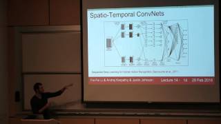
Andrej Karpathy covers video understanding from dense trajectories to 3D convolutions, comparing early fusion, slow fusion, and two-stream architectures. On a 1M-video sports dataset, single frames alone hit 59.3% accuracy, with motion adding only 1.6%. The lecture then introduces unsupervised learning: autoencoders with reconstruction loss and generative adversarial networks.
Chapters
In terms of administrative items, um, everyone should be done with assignment 3 now. If you're not done, I think you're late and you're in trouble. Uh, milestone grades will be out very soon. We're still getting through them and they're basically I think done, but we have to double-check a few things and we'll send them out. Okay. So in terms of reminding you where we are in the class, uh, last class we looked very briefly at segmentation. We looked at some soft attention models. Soft attention models are a way for, uh, selectively paying attention to different parts of the image as you're processing it with something like a recurrent neural network. So it allows you to selectively pay attention to some parts of the scene and enhance those features. And we also talked about spatial transformer, which is this very nice way of basically, in a differentiable way, cropping parts of an image or of some features either in an affine region or in any kind of warped shape or anything like that. So a very interesting kind of piece that you can slot into your neural network architectures. So today we'll talk about videos specifically. Now, in image classification, you should be familiar by now with the basic ConvNet setup. You have an image that comes in and we're processing it to, for example, classify it. In the case of videos, we won't have just a single image, but we'll have multiple frames. So if this is an image of 32 by 32, we'll actually have an entire video of frames. So 32 by 32 by t, where t is some time extent. Okay? So before I dive into how we approach these problems with convolutional neural networks, I'd like to talk very briefly about how we used to address them before ConvNets came about using feature-based methods. So some of the most popular features right before convolutional networks kind of became very, popular were these Dense Trajectory Features developed by Heng Wang et al. And I'd just like to give you a brief taste of exactly how these features worked, um, because it's kind of interesting and they inspire some of the later developments in terms of how convolutional networks actually operate over videos. So in Dense Trajectories, what we do is we have this video that's playing and we're going to be detecting these key points that are good to track in a video and then we're going to be tracking them and you end up with all of these little tracklets that we actually track across the video, and then lots of features about those tracklets and about the surrounding features get accumulated in the histograms. So just to give you an idea about how this worked, there's basically 3 steps roughly. Uh, we detect feature points at different scales in the image. I'll tell you briefly about how that's done in a bit. Then we're going to track those features over time using optical flow methods. Optical flow methods, I'll explain very briefly. They basically give you a motion field from one frame to another, and they tell you how the scene moved from one frame to a next, to next frame. And then we're going to extract a whole bunch of features, but importantly, we're not just going to extract those features at fixed positions in the image, but we're actually going to be extracting these features in the local coordinate system of every single tracklet. And so these histogram of gradients, histogram of flows, and MBH features, we're going to be extracting them in the coordinate system of a tracklet. And so HOG here, we saw histograms of gradients in two-dimensional images. Are basically, um, generalizations of that to, uh, videos. And so that's the kind of things that people use to encode little spatial-temporal volumes. So in terms of the keypoint detection part, um, there's been quite a lot of work on exactly how to detect good features and videos to track. And intuitively, you don't want to track regions in the video that are too smooth because you can't lock onto any visual feature. And so there are ways for basically getting a set of points that are easy to track in a video. So there are some papers on this. So you detect a bunch of features like this. Uh, then you run optical flow algorithms, uh, on these, uh, videos. So an optical flow algorithm will take a frame and a second frame, and it will solve for a motion field, a displacement, uh, vector at every single position into where it traveled or how the frame moved. And so here are some examples of optical flow results. Um, basically, here every single pixel is colored by a direction. In which that part of the image is currently moving in the video. So for example, this girl has— is all yellow, meaning that she's probably translating horizontally or something like that. The two most common methods for using optical flow or for computing it, or at least maybe one of the most common ones here, is Brox from Brox and Malik. That's the one that is kind of like a default thing to use. So if you are computing optical flow in your own project, I would encourage you to use this large displacement optical flow method. So using this optical flow, we have all these key points. Using optical flow, we know also how they move. And so we end up tracking these little tracklets of maybe roughly 15 frames at a time. So we end up with these half a second roughly tracklets through the video. And then we encode regions around these tracklets with all these descriptors. And then we need to accumulate all these visual features into histograms. And people used to play with different kinds of like, how do you exactly chunkate, video spatially because we're going to have a histogram, an independent histogram in every one of these bins. And then we're going to basically create all these histograms per bin with all of these visual features. And all of this then goes into an SVM. And that was kind of the rough layout in terms of how people addressed these problems in the past.
Question?
[Speaker:AUDIENCE] How are you defining a tracklet? [Speaker:ANDREJ KARPATHY] Yeah, so tracklet, just think of it as it's going to be 15 frames. And it's just xy positions, so 15 xy coordinates.
That's a tracklet.
And then we extract features in the local coordinate system. Now, in terms of how we actually approach these problems with convolutional neural networks, so you may recall AlexNet. On the very first layer, we receive an image that is, for example, 227 by 227 by 3, and we're processing it with 96 filters that are 11 by 11 applied at stride 4. And so we saw that with an AlexNet, this results in a 55 by 55 by 96 volume. Um, in which we actually have all these responses of all the filters at every single spatial position. So now, what would be a reasonable approach if you wanted to generalize a convolutional network into a case where you don't just have a 227 by 227 by 3, but you maybe have 15 frames that you'd like to encode? So you have an entire block of 227 by 227 by 3 by 15 that's coming into a convolutional network, and you're trying to encode both the spatial and temporal patterns in the— inside this little block of volume. So it would be like one idea for how to change a convolutional network or generalize it to this case. Okay.
[Speaker] This is what we were doing initially for our project. So we downsampled each of the image and create a 4x4 grid and place the images side by side.
[Speaker:ANDREJ KARPATHY] Okay. That's interesting. So you're saying that you basically took 4 frames and you arranged them as like Blocks, right? Okay. [Speaker:AUDIENCE] Or you can even like, forecast for the 16 frames. [Speaker:ANDREJ KARPATHY] That's interesting.
Okay.
I would expect that to not work very, very well. So the problem with that is— that's kind of interesting. Basically, all these neurons, they're looking at only a single frame. And then by the end of the ConvNet, you end up with neurons that are looking at larger and larger regions in the original image. So eventually, these neurons would see all of your input, but they would not be able to very easily relate the little spatial temporal patch in this image. So I'm not sure actually if that's a really good idea. [LAUGHTER] Okay, go ahead.
[Speaker] Could you tie LSTM into this or something?
[Speaker] Could you tie an LSTM into it? I think so. We'll get to some methods that do something like that. Go ahead.
[Speaker] You could just stack in time just like similar to how you do RGB for your convolutional kernel.
[Speaker] Okay, so that's maybe a good idea. So maybe you would take— so right now we have 3 channels, and maybe you will take these frames and you'll actually just stack them across channels. So you'll end up with 45 channels effectively, and you could put a ConvNet on that. So that's something that I'll get to, I think, in the end. You could do that. I don't think it's the best idea at all.
[Speaker:AUDIENCE] Wouldn't you want to share the parameters across— for each convolutional filter across different time frames so that— because things in one time frame are probably similar to things in another time frame.
[Speaker:ANDREJ KARPATHY] Yes. So you're saying that things in one slice of this time are— you want to extract similar kinds of features in one time than a different time, similar to the motivation of doing it, uh, sharing weights spatially because features here are useful down there as well. So you have the same kind of property where you'd like to share weights in time, not only in space. Okay. So building on top of that idea, the basic thing that people usually do when they want to apply convolutional networks on videos is they extend these filters not only— so you don't only have filters in space, but you also have these filters and you extend them small, amounts in time. So before we have 11 by 11 filters, so now we're just going to have 11 by 11 by t filters, where t is some small temporal extent. So say for example, we can use a 2 up to 15 in this particular case. So for example, if t was 3, then we have 11 by 11 by 3 filters, and then by 3 because we have RGB. And so basically these filters are now— you're thinking of sliding filters not only in space and carving out an entire activation map, but you're actually sliding filters not only in space but also in time, and they have a small finite temporal extent in time, and you end up carving out an entire activation volume. Okay, so you are introducing this time dimension into all your kernels and into all your volumes. They just have an additional time dimension along which we're performing the convolutions. So that's usually how people extract the features. And then you get this property where, say, t is 3 here, and so then when we do the spatial-temporal convolution, we end up with this parameter sharing scheme going in time as well, as you mentioned. Basically, we just extend all the filters in time, and then we do convolutions not only in space but also in time. We end up with activation volumes instead of activation maps. Some of these approaches were proposed quite early on. For example, one of the earlier ones for— in a context of activity recognition is maybe from 2010. The idea here was that this is just a convolutional network, but instead of getting a single input of 60 by 40 pixels, we are getting in fact 7 frames of 60 by 40, and then their convolutions are 3D convolutions as we refer to them. So these filters, for example, might be 7 by 7, but now by 3 as well. And so you end up with a 3D conv, and, um, these 3D convolutions are applied at every single stage here. Um, similar paper also from 2011 with the same idea. We have a block of frames coming in, and you process them with 3D convolutions. So you have 3-dimensional convolutional filters at every single point in this convolutional network. So this is in 2011. Uh, very similar idea also. So these are from before actually AlexNet. These approaches are kind of like smaller neural networks and convolutional network. So the first kind of large-scale application of this was from this awesome paper in 2014 by Karpathy et al. So this is for processing videos. So the model here on the very right that we called slow fusion, that is the same idea that I presented so far. These are 3-dimensional convolutions happening in both space and time. And so that's slow fusion, as we refer to it, because you're slowly fusing this temporal information just as before we were slowly fusing the spatial information. Now, there are other ways that you could also wire up convolutional networks. And just to give you some context historically, this is— I was in Google Research, and AlexNets just came out, and everyone was super excited because they work extremely well on images. And I was in the video analysis team at Google, and we wanted to run ConvNets on the YouTube videos. And— but it was not quite clear exactly how to generalize, you know, convolutional networks and images to videos. And so we explored several kinds of architectures of how you could actually wire this up. So flow— slow fusion is a 3D conv kind of approach. Early fusion is this idea that someone described earlier where you take a chunk of frames and you just concatenate them along channels. So you might end up with a 227 by 227 by like 45, where everything is just stacked up and you do a single conv over it. So it's kind of like your filters on the very first conv layer have a large temporal extent, but from then on everything else is two-dimensional convolution. So in fact, We call it early fusion because it fused the temporal information very early on in the very first layer, and from then on everything is just 2D conv. You can imagine architectures like late convolution. So here the idea is we take two AlexNets, we place them, say, 10 frames apart. So they both compute independently on these 10 frames apart, and then we merge them much later in the fully connected layers. And then we had a single-frame baseline that is only looking at a single frame of a video. So you can play with exactly how you wire up these models. For the slow fusion model, you can imagine that if you have 3-dimensional kernels now in the first layer, you can actually visualize them. And these are the kinds of features you end up learning on videos. So these are basically the features that we're familiar with, except they're moving because now these filters are also extended a small amount in time. So you have these little moving blobs. And some of them are static and some of them are moving. And they're basically detecting motion on the very first layer. And so you end up with nice moving volumes. Go ahead. How much— how deep in time do we go for the filters? Does it still apply that we should try to make it as small as possible? Yeah. So your question is, how much do we extend this in temporal length for the filters? We'll get to that. And I think the answer is probably yes. Just as in spatial, it works better if you have smaller filters and you have more depth. The same applies, I think, in time. And we'll see an architecture that does that in a bit. Go ahead.
What exactly is the output of the full content? Like, what vector are you expecting at the very end? I see.
So in these cases— oops. In these cases, we're expecting the same. We're just classifying every single— so we have a video, and we're still classifying a fixed number of categories at every single frame. But now your prediction is not only a function of that single frame but also a small number of frames on both sides. So maybe your prediction is actually a function of, say, 15 frames, half a second of video. So we end up with fun moving filters. In this paper, we also released a video dataset of 1 million videos and 500 classes. Just to give you context for why this is actually— it's kind of difficult to work with videos in, um, right now, I think, because problem right now, I think, is that there's not too many very large-scale datasets, like on the order of millions of very varied images that you see in ImageNet. There are no really good equivalents of that in the video domain. And so we tried with this sports dataset back in 2013, but I don't think it actually— we fully achieved that. And I think we're still not seeing very good, really large-scale datasets in videos. And that's partly why we're also slightly discouraging some of you from working on this on projects because you can't pre-train these very powerful features because the datasets are just not quite there. Another kind of interesting things that you see, and this is why we also sometimes caution people from working on videos and getting very elaborate very quickly with them, is because sometimes people, they think they have videos and they get very excited. They want to do 3D convolutions, LSTMs, and they just think about all the possibilities that open up before them. But actually, it turns out that single-frame methods are a very strong baseline, and I would always encourage you to run that first. So don't worry about the motion in your video and just try single-frame networks first. So for example, in this paper, we found that a single-frame baseline was about 59.3% classification accuracy on our dataset. And then we tried our best to actually take into account small local motion, but we ended up only bumping that by about 1.6%. So, all this extra work, all the extra compute, and then you ended up with relatively small gains, and I'm going to try to tell you why that might be. But basically, video is not always as useful as you might intuitively think. So, here are some examples of predictions that we— these are different datasets of sports and our predictions, and I think this highlights slightly why adding video might not be as helpful in some settings. So, in particular here, if you're trying to distinguish sports and think about, trying to distinguish, say, tennis from swimming or something like that. It turns out that you actually don't need very fine local motion information if you're trying to distinguish tennis from swimming, right? Lots of blue stuff, lots of red stuff. Like, the images actually have a huge amount of information, and so you're putting in a lot of additional parameters and trying to go after these local motions. But in most, uh, in most classes, actually, these local motions are not very important. They're only important if you have very fine-grained categories where the small motion actually really matters a lot. And so a lot of you, if you have videos, you'll be inclined to use, uh, spatio-temporal crazy video networks, but think very hard about, is that locomotion extremely important in your setting? Because if it isn't, you might end up with results like this where you put in a lot of work and it might not work extremely well. Let's look at some other, uh, video classification, uh, convolutional networks. So this is a paper from 2015. It's relatively popular. It's called C3D. And the idea here was basically VGG network has this very nice architecture where it's 3x3 conv and 2x2 pool throughout. So the idea here is that basically let's do the exact same thing but extend everything in time. So going back to your point, you want very small filters. So this is everything is 3x3x3 conv, 2x2x2 pool throughout the architecture. So it's a very simple kind of VGGNet in 3D, uh, kind of approach and that works reasonably well and you can look at this paper for reference. Uh, another form of approaches actually that works quite well is from, uh, Karan Simonyan in 2014. Karan Simonyan, by the way, is of VGGNet fame. Uh, he's a person who came up with the VGGNet. He also has a very nice paper on video classification. And the idea here is that he didn't want to do 3-dimensional convolutions because it's kind of painful to have it implemented or find it and so on. So he only used 2-dimensional convolutions. But the idea here is that we have 2 ConvNets looking at an image and the other one is looking at optical flow of the video. So both of these are just images, but the optical flow basically tells you how things are moving in the, in the image. And so both of these are just kind of like a VGGNet-like or AlexNet-like ConvNet, one of them on optical flow, one of them on the image. And you extract optical flow with, say, the Brox method that I've shown you before. And then you let— you fuse that information very late in the end. So both of these come up with some idea about what they are seeing in terms of the classes in the video, and then you fuse them, and there are different ways of fusing them. And so they found, for example, that if you just use a spatial ConvNet, so it's only looking at images, you get some performance. If you use a ConvNet on just the optical flow, it actually performs even slightly better than just looking at the raw images. So optical flow actually here in this case contains a lot of information. And then if you fuse them, you actually end up performing even better. Now, an interesting point to make here, by the way, is that if you have this kind of architecture, especially here, complex— this 3x3x3 filters, you might imagine that actually you would think that— I mean, why does it help to actually put in optical flow? You'd imagine that in this end-to-end framework, we're hoping that these ConvNets learn everything from scratch. In particular, they should be able to learn something that simulates the computation of computing optical flow. And it turns out that that might not be the case because sometimes when you compare video networks on only the raw pixels and then you add optical flow, it works better. And so I think the reason for that is probably comes back to actually data. Since we don't have enough data, we have small amount of data, I think you actually probably don't have enough data to actually learn very good optical flow-like features. And so that would be my particular answer why actually hardcoding optical flow into the network is probably helping out in many cases. So if you guys are working on your projects with videos, I would encourage you to actually try maybe this kind of architecture where you extract optical flow and then you pretend that it's an image. And you put ConvNets on it and you merge it. And so that seems like a relatively reasonable approach. Okay. So, so far we've only talked about little local information in time, right? So we have these little piece of like movement, say of like half a second, and we're trying to take advantage of it to do better classification. But what happens if you have videos that actually have much longer temporal, um, temporal kind of dependencies that you'd like to model? So it's not only that the local motion is important, but actually there are some events throughout the video that are much larger in timescale than your network. And they actually matter. So event 2 happening after event 1 could be very indicative of some class, and you'd like to actually model that with a neural network. So what are the kinds of approaches that you might think for trying to actually, you know, how would you modify the architecture to actually model these kinds of much longer-term events? Go ahead.
Attention model?
Okay. So attention model perhaps. So you'd maybe like to have an attention over, You're trying to classify this entire chunk of video and maybe you'd like to have attention over different parts of the video.
Yeah.
Sensible idea. Go ahead. Sometimes we look at images at very different scales. We could do the same thing in time where we just skip frames. Um, I see. Yeah, that's a good idea. So you're saying that we have these multi-scale approaches where we process images on very low detail level, but also sometimes we resize the images and process them on the global level. And so maybe the frames we can actually like speed up the video and put a ConvNet on that. I don't think that's very common, but it's a sensible idea, I think.
Yeah, it's good.
So the problem roughly is that basically this temporal extent is maybe sometimes too short. It doesn't span entire many seconds. So how do we make architectures that are a function of much longer timescales in their prediction?
Good.
[Speaker] Could you include a hidden state like a recurrent neural network? [Speaker:ANDREJ KARPATHY] OK. Yeah, so one idea here is we have this video, and we have different classes that we'd like to predict at every single point in time. But we want that prediction to be a function not only of a little chunk of 0.5 seconds, but actually of much longer time extents. And so the idea that is sensible is you actually use recurrent neural networks somewhere in the architecture, because recurrent networks allow you to have infinite context in principle over everything that has happened before you up till that time. So actually, if you go back to this paper that I've already shown you in 2011, it turns out that they have an entire section where they take this and they actually have an LSTM that does exactly that. So this is a paper from 2011 using 3D Conv and LSTMs way before they were cool. In 2011. And so this paper basically has it all. They model little local motion with 3D Conv, and they model global motion with LSTMs. And so they put LSTMs on, say, the fully connected layers. So they string together fully connected layers with this recurrence. And then when you're predicting classes at every single frame, you have infinite context. And so this paper is, I think, quite ahead of its time. And it basically has it all, except it's only cited 65 times. I'm not sure why it's not more popular. I think people— I don't know. But basically, this is a way ahead of its time paper that recognized both of these and actually used LSTMs way before I even knew about them. So since then, there are several more recent papers that actually kind of take this similar approach. So in 2015, by Geoff Donahue et al. from Berkeley, the idea here is that you have video, and you'd like to again classify every single frame. But they have these ConvNets that look at individual frames, but then they have also LSTMs that string this together temporally. A similar idea also from a paper from, I think this is Google. And so the idea here is that they have optical flow and images, both are processed by ConvNets, and then again you have an LSTM that merges that over time. So again, this, this combination of local and global. So, so far we've looked at kind of two architectural patterns in accomplishing video classification that actually takes into account temporal information. Modeling local motion, which for example we extend 3D Conv where we use optical flow, or look more global motion where we have LSTM that string together sequences of learning timestamps or fusions of the two. Now actually, I'd like to make the point that there's another cleaner, very nice, interesting idea that I saw in the recent paper and that I like much more. And so here's basically the rough picture of what things look like right now. We have some video and we have a 3D ConvNet say that is using optical flow maybe, or it's using 3D Conv or both on a chunk of frame, chunk of your data. And then you have RNNs on the top on the fully connected layer or something like that that are doing the long-term modeling. And so kind of what's kind of not very nice or unsettling about this is that there's kind of this ugly asymmetry about these components. So you have these part— these neurons inside the 3D ConvNet are only a function of some small local chunk of video. And then you have these neurons on the very top that are a function of everything in the video. Because they're recurrent units that are a function of everything that's become— come before it. And so it's kind of like an unsettling asymmetry or something like that. So there's a paper that has a very clever and neat idea from a few weeks ago that is much more nice and homogeneous in a VGGNet-like style where everything is very nice and homogeneous and simple. And so I don't know if anyone can think of how we could— what we could do to make everything much more cleaner. And I couldn't because I didn't come up with this idea, but I thought it was cool once I read it. Go ahead.
Maybe you could reverse and do the RNN before the ConvNet.
Interesting. You want to do the RNN before the ConvNet actually starts processing the images? I'm not sure what that would give you. So you would have RNNs on the raw pixel information and then ConvNets on top of it somehow? You would certainly have neurons that are a function of everything. But it's not clear what the LSTM would be doing in that case. Like, would it be blurring the pixels? It's too low-level, probably, processing at that point.
Good? So it seems like one of the problems is that in video, there's so much duplicate information between two frames that, like, there's a lot of redundancy if you're only looking at a few frames. So you could have maybe, like, an ensemble of confidence that looks at different, like, temporal resolutions. So this confidence is looking every frame, right? But you could have— another ConvNet that's looking like every 2 frames, every 4 frames, every 8 frames, and then you could feed all of those into the RNet.
I see. Uh, so your idea is that I think it's similar to what someone pointed out where you take this video and you work on multiple scales of that video. So you speed up the video and you slow down the video and then you have 3D ConvNets on different, um, temporal like, uh, speeds or something like that. I think it's a sensible idea. Yeah?
Why don't you just do background subtraction and get only the stuff that's sort of interesting to look at?
Could you do background subtraction, only look at things that are interesting to look at? I think that's a reasonable idea. I think it kind of goes against this idea of having end-to-end learning because you're introducing like this explicit computation that you think is useful. Yeah. Simplifying learning basically. I see. Yeah. Good. Could we have weight sharing between the 3D ConvNet and the RNN? Can we have weight sharing between the 3D ConvNet and the RNN? Um, that's interesting. I'm not 100% sure because the RNN is just a hidden state vector and you're doing matrix multiplies and things like that. But in the Conv layers, we have this like spatial structure. So I'm not actually sure how the sharing would work. Um, but yeah, maybe.
Okay.
So the idea is that we're going to, uh, let's see, we're going to get rid of the RNN. We're going to basically take a ConvNet and we're going to make every single neuron in that ConvNet be a small recurrent neural network. Like every single neuron becomes recurrent in the ConvNet. Okay? So the way this will work, and I think this is beautiful, uh, but their picture is kind of, uh, kind of ugly. So I'm not sure if this makes, makes sense. So let me try to explain this in a slightly different way. What we'll do instead is, so in a normal ConvNet, we have a conv layer somewhere in the neural network, and it takes input from below the output of a previous conv layer or something like that. And we're doing convolutions over this to compute the output at this layer, right? So the idea here is, we're going to make every single convolutional layer a kind of a recurrent layer. And so the way we do that is we, just as before, we take the input from below us and we do convs over it, but we also take our previous output from the previous time, time step of this conv layer's output. So that's this conv layer from previous time step in addition to the current input at this time step. And we do convolutions over both this one and that one. And then we kind of have, um, you know, we've done conv and we have these activations from, uh, current input, and we have activations from our previous output, and we add them up or something like that. We do a recurrent neural network-like merge of those two to produce our output. And so we're a function of the current input, but we're also a function of our previous activations, if that makes sense. And so what's very nice about this is that we're in fact only using two-dimensional convolutions here. There's no 3D conv anywhere because both of these are width by height by depth. Right, so the previous conv volume is just width, height, depth from the previous layer, and we are width, height, depth from previous time. And so both of these are two-dimensional convolutions, but we end up with kind of like recurrent process in here. And so one way to see this also with recurrent neural networks, which we've looked at, is that you have this recurrence where you're trying to compute your hidden state, and it's a function of your previous hidden state and the current input x. And so we looked at many different ways of actually wiring up that recurrence. So there's a vanilla RNN, or an LSTM, or there's a GRU, which— a GRU is a simpler version of an LSTM, if you recall, but it almost always has similar performance to an LSTM. So GRU has slightly different update formulas for actually performing that recurrence. And so what they do in this paper is basically they take the GRU because it's a simpler version of an LSTM that works almost just as well, but instead of every single matrix multiply, it's kind of like replaced with a conv, if you can, um, if you can imagine that. So every single matrix multiply here just becomes a conv, So we convolve over our input and we convolve over our output, and that's the before and the below, and then we combine them with the recurrence just as in the GRU to actually get our activations. And so before, it looked like this, and now it basically just looks like that. So, uh, we don't have some parts being infinite in extent and some parts finite. We just have this RNN ConvNet where every single layer is recurrent. It's computing what it did before, but also it's a function of its previous outputs. And so this RNN-ConvNet is a function of everything. Um, and it's very kind of uniform. It's kind of like a VGGNet. You just do 3x3 conv, 2x2 max pool, and you're recurrent, and that's it. Maybe that's just the answer. It's the nicest, simplest thing. So in summary— whoops, where's my summary? Um, so if you'd like to use spatio-temporal convolutional networks in your projects and you're very excited because you have videos, the first thing you should do is stop and you should think about whether or not you really need to process local motion or global motion, or if motion is really important to your classification task. If you really think motion is important to you, then think about whether or not you need to model local motions. Are those important, or are the global motions very important? Based on that, you get a hint of what you should try, but you always have to compare that to a single-frame baseline, I would say. And then you should try using optical flow because it seems that if you especially have smaller amount of data, it actually is very important. It's like a very nice signal to actually encode that and explicitly specify that optical flow is a useful feature to look at. And you can try this GRU-RCN network that I've shown you just now, but I think this is too recent and experimental, so I'm actually not sure if I can fully endorse this or if it works. It seems like it's a very nice idea, but it hasn't kind of been proven yet. And so that's kind of like the rough layout of how people process videos in the field. I don't know if there are any questions because Justin is going to come next. Good?
I'm wondering if architectures like GRU, R-CNN that you last mentioned have been used for NLP.
Architecture like GRU, R-CNN. So this one, has it been used for NLP? That's a good question. I don't think so. I'm not super duper expert on NLP, but I haven't seen this idea before. So I would guess that I haven't seen. Yeah, I'm not sure. I don't think so. Go ahead.
I have an answer for that. There is a model really similar to this, but it's more similar to the half the scene in the bottom, RN on the top. It's from Yong Kim, who is working at Harvard with Sasha right now.
So does it look more like this then? Yes. Yeah, OK. Yeah. OK.
Question? Do people ever do— like networks that take into account the audio also?
[Speaker:ANDREJ KARPATHY] Do people take into account networks that also take in audio and somehow consider it on the side with the video? I would say that that's definitely something people would want to do. You don't see too many papers that do both of them just because people like to kind of isolate these problems and tackle them maybe not jointly. But certainly if you're in a company and trying to get something working in a real system, you would do something like that. But I don't think that there's anything that you would do— you'd probably do this with a late fusion approach where you have a— whatever works best on videos, whatever works best on audio, and then you merge that somewhere later somehow. But that's certainly something you can do. Yeah, it's a good idea. And with the neural networks, right, it's very simple because you just have a fully connected layer that's looking at the output of both at some point, and then you're classifying as a function of both. Yeah. All right, cool. So we're going to go into unsupervised learning. And I guess we have to—
Yeah, you have to switch places. Yeah, this is our first tag team lecture. Hopefully it works. All right. Can you hear me? Is that hooked up? OK. OK. So I guess for the rest of the lecture, we're going to switch gears completely and entirely and talk about unsupervised learning. So I'd like to make a little bit of a contrast here that First, uh, we're gonna talk about some sort of basic definitions around unsupervised learning, and then we're gonna talk about, uh, two different sort of ways that unsupervised learning has recently been attacked by deep learning people. Um, so in particular, we're gonna talk about autoencoders and then this idea of adversarial networks. And I guess I need my clicker. Right. So pretty much everything we've seen in this class so far is, um, supervised learning. So the basic setup behind pretty much all supervised learning problems is that we assume that our dataset has sort of— each data point has sort of two distinct parts. We have our data x, and then we have some label or output y that we want to produce from that input. And the whole goal in supervised learning is to learn some function that takes in our input x and then produces this output or label y. And if you really think about it, pretty much almost everything we've seen in this class is some instance of this supervised learning setup. So for something like image classification, X is an image and then Y is a label. For something like object detection, X is an image and then Y is maybe a set of objects in the image that you want to find. Y could be a caption and then we look at captioning. X could be a video and now Y could be either a label or a caption or pretty much anything, anything. So I just want to make the point that supervised learning is this very, very, very powerful and generic framework. That encompasses, uh, everything we've done in the class so far. Um, and the other point is that supervised learning actually makes systems that work— systems that work really well in practice and is very useful for practical applications. Um, unsupervised learning I think is a little bit more of an open research question at this point in time. So it's really cool. Um, I think it's really important for solving AI in general, but at this point it's maybe a little bit more of a research-focused type of area. Um, it's also a little bit less well-defined. So if in unsupervised learning, we generally assume that we have just data, we only have X, we don't have any Y. And the, the, the goal of unsupervised learning is to do something with that data X. And the something that we're trying to do really depends on the problem. Uh, so some— so in general, we hope that we can discover some type of latent structure in the data X without explicitly knowing anything about the labels. So some classical examples that you might have seen in previous machine learning classes would be things like clustering. So something like k-means where X is just a bunch of points and we discover structure by classifying them into clusters. Um, uh, some other classical examples of unsupervised learning would be something like principal component analysis where X is just this, uh, some bunch of data and we want to discover some low-dimensional representation of that input data. So unsupervised learning is this really sort of cool area, but a little bit more problem-specific and a little bit less well-defined than supervised learning. So two things that— two architectures in particular that people in deep learning have done for unsupervised learning are these ideas, uh, is this idea of an autoencoder. Um, we'll talk about sort of traditional autoencoders that have a very, very long history. We'll also talk about variational autoencoders, which are this sort of new school Bayesian twist on them. We'll also talk about some generative adversarial networks that actually are this really nice idea that let you generate images and model, uh, sample from natural images. So the idea with an autoencoder is, is pretty simple. Um, we have our inputs x, which is some data, and we're gonna pass this input data through some kind of encoder network. To, to produce some features, uh, some latent features z. So this you could think— this stage, uh, you could think of a little bit like a learnable principal component analysis where we're going to take our input data and then convert it into some other feature representation. So those, uh, many times these x's will be images like these CIFAR-10 images shown here. Um, so this, this encoder network could be something very complicated. So for something like PCA, it's just a simple linear transform. But in general, this might be a fully connected network. Um, originally, uh, sort of maybe 5 or 10 years ago, this was often a single layer fully connected network with sigmoid units. Now it's often a deep, uh, deep network with ReLU units, and this could also be something like a convolutional network. Uh, right. So we also have this idea that, uh, z, the, the features that we are, that we learn are usually smaller in size than x. So we want z to be some kind of useful features about the data x. So we, um, we don't want the network to just, uh, transform the net— transform the data into some useless representation. We want to force it to actually crush the data down and summarize its statistics in some useful way that could hopefully be useful for some downstream processing. But, um, the problem is that we don't really have any explicit labels to, to use for this downstream processing. So instead, we need to invent some kind of a surrogate task that we can use using just the, just the data itself. So the, the surrogate task that we often use for autoencoders is this idea of reconstruction. So since we don't have any Ys to learn a mapping, instead, we're just gonna try to reproduce the data X from those features Z. And especially if those features Z are smaller in size, then hopefully that'll force the network to act— to summarize the, to summarize the useful statistics of the input data, um, and hopefully discover some useful features that could be, um, one, useful for reconstruction, but more generally, maybe those features might be useful for some other tasks, uh, if we later get some supervised data. So, uh, again, this decoder network could be pretty complicated. Uh, when autoencoders first came about, oftentimes these were just simple— either a simple linear network or a small sigmoid network. but now they can be deep ReLU networks, and oftentimes these will be, um, I decided upconvolutional is a good term. So it's nice and small and fits on the slides. So oftentimes this decoder nowadays will be one of these upconvolutional networks that takes your features that are again are smaller in size than your input data and kind of blows it back up in size to reproduce your original data. Um, and I'd like to make the point that these things are actually pretty easy to train. So on the right here is a quick example that I just cooked up in Torch. So this is a 4-layer encoder, which is a, a convolutional network, and then a 4-layer decoder, which is an upconvolutional network. And you can see that it's actually learned to reconstruct the data pretty well. Um, another thing that you'll sometimes see is that these encoder and decoder networks will sometimes share weights, um, with— just sort of as a regularization strategy, and with this intuition that these are opposite operations, so maybe it might make sense to try to use the same weights for both. So just as a concrete example, um, if you're in— if you think about a fully connected network, then maybe your input data has some dimension D, and then your latent data Z will have some smaller dimension H. And if this encoder was just a fully connected network, then the weights would just be this matrix of D by H. And now when we want to do the decoding and try to reconstruct the original data, then that— we're mapping back from H back to D. So, uh, we can just reuse the same weights in these two layers if we just take a transpose of the matrix. So when we're training this thing, we need some kind of a loss function that we can use to compare our, our reconstructed data with our original data. Um, and then once, uh, and oftentimes we'll see L2, a simple like L2 Euclidean loss to, to train this thing. So once we've chosen our encoder network and once we've chosen our decoder network and chosen a loss function, then we can train this thing just like any other normal neural network. Where we get some data, we pass it through to encode it, we pass it through to decode it, we compute our loss, we backpropagate, and everything's good. So once we train this thing, then oftentimes we'll take this decoder network that we spent so much time learning and we'll just throw it away. Um, which seems kind of weird, but the reason is that reconstruction on its own is not such a useful task. So instead, we want to apply these networks to some kind of actually useful task. Which is probably a supervised learning task. So here the setup is that we've learned this encoder network, which hopefully from all this unsupervised data has learned to, has learned to compress the data and extract some useful features. And then we're going to use this encoder network to initialize part of a larger supervised network. And now if we actually do have access to maybe some smaller dataset that has some labels, then hopefully this, most of the work here could have been done by this unsupervised training at the beginning. and then we can just use that to initialize this, this bigger network and then fine-tune the whole thing with hopefully a very small amount of supervised data. So this is kind of the dream of unsup— one of the dreams of unsupervised feature learning, that you have this really, really large dataset of— with no labels. You can just go on Google and download images forever, and it's really easy to get a lot of images. Um, the problem is that labels are expensive to collect. So you'd want some system that could take advantage of both a large, huge amount of unsupervised data, and also just a small amount of supervised data. So autoencoders are at least one thing that has been proposed that has this nice property, but in practice, I think it tends not to work too well, which is a little bit unfortunate because it's such a beautiful idea. Um, another thing that I should point out, uh, almost a bit of a, as a side note that if you go back and read the literature on these things, um, from maybe the mid-2000s, uh, in the last 10 years, then people had this funny thing called greedy layer-wise pre-training that they used for training autoencoders. And here the idea was that, um, at the time in 2006, training very deep networks was, was challenging. And, uh, if you— you can find quotes in papers like this that say that even when you have maybe 4 or 5 hidden layers, it was extremely challenging for people in those days to train deep networks. Um, so to get around that problem, they instead had this paradigm where they would try to train just one layer at a time. And they used this, this thing that I don't want to get too much into called a restricted Boltzmann machine, which is a type of graphical model. And they would use these restricted Boltzmann machines to kind of train these two— these little layers one at a time. So first we would have our input image of maybe size— of size W1. And this would be maybe something like PCA or some, some other kind of fixed transform. And then we would hopefully learn, um, using a restricted Boltzmann machine, some kind of relationship between those first layer features and some higher layer features. Um, when— once we— once we learn this layer, we would then freeze it and learn another restricted Boltzmann machine on top of those features connecting it to the next layer of features. Um, so by using this type of approach, it let them train just one layer at a time in this sort of greedy way. And that let them hopefully find a really good initialization for this larger network. So after this, uh, greedy pre-training stage, they would stick the whole thing together into this giant autoencoder and then fine-tune the autoencoder jointly. So, um, nowadays we don't really need to do this, um, with things like ReLU and proper initialization and batch normalization and slightly fancier, fancier optimizers. This type of thing is not really necessary anymore. Um, so as an example, um, On the previous slide, we saw this 4-layer convolutional deconvolutional autoencoder that I trained on CIFAR. And this is just fine to do, um, using all these modern neural network techniques. You don't have to mess around with this, uh, greedy layer-wise training. So this is not something that really gets done anymore, but I thought we should at least mention it since you'll probably encounter this idea if you lo— read back in the literature about these things. So the basic idea around autoencoders is I think pretty simple. It's this beautiful idea where we can just use a lot of unsupervised data to hopefully learn some nice features. Um, unfortunately that doesn't work, but that's okay. Um, but there's maybe some other nice type of task we would want to do with unsupervised data. Uh, question first.
Sorry, could you just explain how exactly you train the weights again? Um, so you take your input data and you compute a loss at the end.
What does that mean? —your output and then— Yeah, so the question is what's going on here, right? So this is maybe— you could think about a 3-layer neural network. So our input is going to be the same as the output. So we're just hoping that this is a neural network that will learn the identity function. But that's a really— and in order to learn the identity function, we have some loss function at the end, something like an L2 loss that is encouraging our input and our output to be the same. Um, and learning the identity function is probably a really easy thing to do, but instead we're gonna force the network to not take the easy route, and instead hopefully rather than just regurgitating the data and learning the identity function in the easy way, instead we're gonna bottleneck the representation through this hidden layer in the middle. So then, um, it's gonna learn the identity function, but in the middle it— the network is gonna have to squeeze down and summarize and compress the data. And hopefully that compression will give rise to features that are useful for other tasks. Is that maybe a little bit more clear? OK. Question? Don't we already know that PCA is the answer for this problem? So the claim was that PCA is just the answer for this problem. So it's true that PCA is optimal in certain senses if you're only allowed to do maybe a one-layer type of if your encoder and your decoder are just a single linear transform, then indeed PCA is optimal in some sense. Um, but if your encoder and decoder are potentially larger, more complicated functions that are mo— maybe multi-layer neural networks, um, then it— then maybe PCA is no longer the right solution. Another point to make is that PCA is only optimal in certain senses, um, particularly talking about L2 reconstruction. Um, but in practice, we don't actually care about reconstruction. We're just hoping that this thing will learn useful features for other tasks. So, uh, in practice, and we'll see this a bit later, that people don't always use L2 anymore because L2 is maybe not quite the right loss for actually learning features. Yeah.
What is the loss function for those, uh, RBM layers?
Um, so the RBM layer is this, uh, is, is this kind of generative model of the data, of data, where you imagine that you have sort of two sequences of bits, and you want to do this generative modeling of the, of the two things. So then you need to, uh, get into quite a lot of Bayesian statistics to figure out exactly what the loss function is. But it ends up being something like log likelihood of the data, um, with these latent states that you don't observe. And that's actually a cool idea that we will sort of revisit in the variational autoencoder. So one of the, one of the problems with this traditional autoencoder is that it's hoping to— it can learn features, that's, that's a cool thing. But there's this other thing that we would like to not just learn features but also be able to generate new data. Um, a cool task that we could potentially learn from unsupervised data is that hopefully our model could slurp in a bunch of images, and after it does that, it sort of learns what natural images look like. And then after it's learned this distribution, then it could hopefully spit out sort of fake images that look like the original images but are fake. And, uh, this is maybe not a, a task which is directly applicable to things like classification, but it seems like an important thing for AI that humans are pretty good at looking at data and summarizing it and kind of getting the idea of what a dataset looks like. So hopefully if our models could also do this sort of task, then hopefully they'll have learned some, some useful summarization or some useful statistics of the data. So the variational autoencoder is this kind of neat twist on the original autoencoder that lets us hopefully, um, actually generate novel images from our learned data. So here we need to dive into a little bit of Bayesian statistics. So this is something that we haven't really talked about at all in this class anymore, but— or up to this point, but there's this whole other side of machine learning that doesn't do neural networks and deep learning, but thinks really hard about probability distributions and how, um, probability distributions can fit together to generate datasets and then reason probabilistically about your data. Um, and this type of paradigm is really nice because it lets you sort of state explicit probabilistic assumptions about how you think your data was generated. And then given those probabilistic assumptions, you try to fit your model to the data that, uh, follows your assumptions. So with the variational autoencoder, we're assuming this, this particular type of method by which our data was generated. So we assume that we— there exists out there in the world some prior distribution which is generating these latent states z. And we then, we assume some conditional distribution that once we have the latent states, we can, uh, sample from some other distribution to generate the data. So the variational autoencoder, it really imagines that our data was generated by this pretty simple process. That first we sample from some prior distribution to get some— to get our z. Then we sample from this conditional to get our x. So the intuition is that x is something like an image and z maybe summarizes some useful stuff about that image. So if these were CIFAR images, then maybe that latent state z could be something like the class of the image, whether it's a frog or a deer or a cat. and also might contain variables about how that cat is oriented or what color it is or something like that. So this is kind of a nice sort of, I think, a pretty simple, pretty simple idea, but makes a lot of sense for how you might imagine image, images to be generated. So the problem now is that we want to estimate these parameters theta of both the prior and the conditional without actually having access to these latent states z. And that's a challenging problem. So to make it simpler, we're going to do something that you see a lot in Bayesian statistics. And we'll just assume that the prior is Gaussian because that's easy to handle. And the conditional will also be Gaussian, but it's going to be a little bit fancier. So we'll assume that it's a Gaussian with diagonal mean and— sorry, diagonal covariance and some mean. But instead, we're just going to But the way that we're going to get those is we're going to compute them with a neural network. So suppose that we had the latent state z for some piece of data, then we assume that that latent state will go into some decoder network, which could be some big complicated neural network. And now that neural network is going to spit out two things. It's going to spit out the mean of the data— it's going to spit out the mean of the data x and also the variance of the data x. So you should think that this looks very much like the top half of a normal autoencoder, that we have this latent state, we have some neural net that's operating on the latent state. But now instead of just directly spitting out the, the data, instead it's spitting out the, the mean of the data and the variance of the data. But other than that, this looks very much like the decoder of the normal autoencoder. So this, this decoder network, um, sort of thinking back to the normal autoencoder, might be a simple fully connected thing or it might be this very big powerful deconvolutional network, and, and both of those are pretty common. So now the problem is that, um, by Bayes' rule, if given the prior and given the conditional, Bayes' rule tells us the posterior that given— so if we want to actually use this model, we need to be able to estimate the latent state from the input data. And the way that we estimate the latent state from the input data, is by writing down this posterior distribution, which is the probability of the latent state z given our observed data x. And using Bayes' rule, we can easily flip this around and write it in terms of our prior over z and in terms of our conditional, um, x given z. Um, the pro— and so we can use Bayes' rule to actually flip this thing around and write it in terms of these three things. So the— after we look at Bayes' rule, we can break down these three terms, and we can see that the The conditional, we just use our decoder network and we easily have access to that. And this prior, again, we have access to the prior because we assumed it's unit Gaussian. So that's easy to handle. But this denominator, this probability of x, it turns out if you, if you work out the math and write it out, this ends up being this giant intractable integral over the entire latent state space. So that's completely intractable. There's no way you could ever perform that integral and even approximating it would be a giant disaster. So instead, we will not even try to evaluate that integral. Instead, we're going to introduce some encoder network that will try to directly, um, perform this inference step for us. So this encoder network is going to take in a data point, and it's going to spit out a distribution over the latent state space. So again, this looks very much, um, looking back at the original autoencoder from a few slides ago, this looks very much the same. as sort of the bottom half of a traditional autoencoder where we're taking in data and now instead of directly spitting out the latent state, we're gonna spit out a mean and a covariance of the latent state. Um, and again, this encoder network might be something, um, might be some fully convolutional network or it might be some deep, uh, convolutional network. So the, the sort of the intuition is that this encoder network will be this separate totally different disjoint function, Um, but we're going to try to train it in a way so that it approximates this posterior distribution that we don't actually have access to. Um, and yeah, this— so once we put all these pieces together, then the— then we can set up, stitch this all together and get— give rise to this variational autoencoder. So once we put these things together, then we have this input data point x, we're gonna pass it through our encoder network, and the encoder network will spit out a distribution over the latent states. Once we have this, this distribution over the latent states, you can imagine, you could imagine sampling from that distribution to get some, some high, some latent state of high probability for that input. Um, then once we have, then once we have some concrete example of a latent state, then we can pass it through this decoder network, which will spit out the probability, um, of which should then spit out the probability of the data again. And then once we have this, this distribution over the data, we could sample from it to actually get something that hopefully looks like the original data point. So this, um, this ends up looking very much like a normal autoencoder where we're taking our input data, we're running it through this encoder to get, um, lat— some latent state, and we're passing it through this decoder to hopefully reconstruct the original data. And when you go about training this thing, it's actually trained in a very similar method as a normal autoencoder. Where we have this forward pass and this backward pass. The only difference is in the loss function. So, um, at the top we have this reconstruction loss rather than being this pointwise L2. Instead, we want this distribution to be close to the true input data. And we also have this, uh, loss term coming in the middle that we want this generated distribution over the latent states to hopefully be very similar to our, um, stated prior distribution that we wrote down at the very beginning. So once you put all these pieces together, you can just train this thing like a normal autoencoder with normal forward pass and backward pass. The only difference is where you put the loss and how you interpret the loss. So any questions about this setup? It's kind of a— we went through it kind of fast. Yeah. Why do you choose a diagonal covariance? The question is, why do you choose a diagonal covariance? And the answer is because it's really easy to work with. There's— but actually people have tried, I think, slightly fancier things too. But that's something you could play around with. Okay. So once we've actually trained this, once we've actually trained this kind of variational autoencoder, we can actually use it to, to generate new data that looks kind of like our original dataset. So here, the idea is that, remember we wrote down this prior that might be a unit Gaussian or maybe something a little bit fancier. But at any rate, this prior is something, some distribution that we can easily sample from. So a unit Gaussian, it's very easy to draw random samples from that distribution. So to generate new data, we'll start by just sort of following this data, this data generation process that we had imagined for our data. So first, we'll sample from our, from our prior distribution over the latent states, and then we'll pass it through our decoder network that we have learned during training. And this decoder network will now spit out a distribution over our data points in the term— in, in terms of both a mean and a covariance. And once we have a mean and a covariance, this is just a diagonal Gaussian. So we can easily sample from this thing again, to generate some data points. Um, so now once, once you train this thing, then another thing you can do is sort of scan out the latent space and amma— and rather than sampling from the latent distribution, instead you just densely sample all the latents from the latent space to kind of get an idea for what type of structure the network had learned. So this is doing exactly that on, on the MNIST dataset. So here we, we trained this variational autoencoder with where z, the latent state, is just a 2-dimensional thing. And now we can actually scan out this latent space. This lat— we can explore densely this 2-dimensional latent space. And for each point in the latent space, pass it through the decoder and use it to generate some image. So you can see that it's actually discovered this very beautiful structure on MNIST digits that sort of smoothly interpolates between the different digit classes. So up here at the left, you see 6s that kind of morph into 0s. As you go down, you see 6s that turn into 7— into maybe 9s and 7s. The 8s are hanging out in the middle somewhere and the 1s are down here. So this latent space actually learned this beautiful disentanglement of the data, um, in this very nice unsupervised way. Um, we, we can also train this thing on a faces dataset and it's the same sort of story where we're just training this two-dimensional variational autoencoder. And then once we train it, we densely sample from that latent space to try to see what has what it has learned. Question? Do people in practice ever force certain variables to be like class labels? So you can say, okay, one of my hidden states is cat, and then I can set that to cat so I can sample specifically like cat images? Yeah. So the question is whether people ever try to force the specific latent variables to have some, some exact meaning. And yeah, there has been some follow-up work that does exactly that. There's a paper called, um, Deep Inverse Graphics Networks from MIT that has— that does exactly this setup. Where they try to force— where they want to learn sort of a renderer as a neural network. So they want to learn to render 3D images of things. So they want to force some of the latent space, some of the variables in the latent space to correspond to the 3D angles of the object and maybe the class and the 3D pose of the object. And the rest of them, it lets it learn for whatever it wants. And they actually have some cool experiments where now they can do exactly as you said. By setting those, those specific values of latent variables, they can render and actually rotate the object. And those are, those are pretty cool. But that's a little, that's, that's a little bit fancier than these faces. But these faces are still pretty cool. You can see it sort of interpolating between different faces in this very nice way. And I think that there's actually a very nice motivation here. And one of the reasons we pick a diagonal Gaussian is that that has the probabilistic interpretation of having independent, uh, that, that the very— that the different variables in our latent space actually should be independent. So I think that helps to explain why there actually is this very nice separation between the axes when you end up sampling from the latent space. It's due to this probabilistic independence assumption embedded in the prior. So this idea of priors is very powerful and lets you sort of bake those types of things directly into your model. So I wrote down a bunch of math, and I don't think we really have time to go through it. But the idea is that sort of classically when you're training generative models, there's this thing called maximum likelihood where you want to maximize the likelihood of your data under the model and then pick the model where that makes your data most likely. But it turns out that if you just try to run maximum likelihood using a normal— using this generative process that we had imagined for the variational autoencoder, then you run into this this giant— you end up needing to marginalize this joint distribution, which becomes this giant intractable integral over the entire latent state space. So that's not something that we can do. So instead, the variational autoencoder does this thing called variational inference, which is a pretty cool idea. And the math is here in case you want to go through it. But the idea is that instead of maximizing the log probability of the data, we're going to cleverly insert this extra constant. And break it up into these two different terms. So we're— this is an exact equivalence that you can maybe work through on your own. But this log likelihood, we can write in terms of this term that we call an ELBO and this other term, which is a KL divergence between two distributions. And we know that KL divergence is always 0. So we know that KL divergence between distributions is nonzero. So we know that this term has to be nonzero. Which means that this, this ELBO term actually is a lower bound on the log likelihood of our data. And notice that in the process of writing down this ELBO, we introduced this additional parameter phi that we can interpret as the parameters of this, of this encoder network that is sort of approximating this hard posterior distribution. So now instead of trying to directly maximize the log likelihood of our data, instead we'll try to maximize this variational lower bound of the data. And because this, this ELBO is a lower bound of the log likelihood, then maximizing the ELBO will also have the effect of raising up the log likelihood instead. And these, these two terms of the ELBO actually have this beautiful interpretation that this one at the, at the front is the expectation over the latent states b— over the latent state space of the probability of x given the latent state space. So if you think about that, that's actually a data reconstruction term. That's saying that if we average over all possible latent states, then we should end up with something that is similar to our original data. And this is— this other term is actually a regularization term. This is the KL divergence between our approximate posterior and between the prior. So this is a regularization that's trying to force those two things together. So in practice, this first term you can approximate with something called the— approximate by sampling. Using this trick in the paper that I won't get into. And this other term, again, because everything is Gaussian here, you can just evaluate this KL divergence explicitly. So I think this is the most math-heavy slide in the class. So that's kind of fun. But actually, it's— so but it's actually— this looks scary, but it's actually just this autoencoder idea where you have a reconstruction and then you have this penalty penalizing you to go back towards the prior. So any, any questions on the variational autoencoder? Okay. So the, the overview of autoencoders is that, um, in general, the idea of an autoencoder is that we want to force a network to try to reconstruct our data, and hopefully this will learn sort of useful representations of the data. Um, for traditional autoencoders, this is used for feature learning, but once we move to variational autoencoders, we make this thing Bayesian so we can actually generate samples that are similar to our data. So then this idea of generating samples from our data is really cool. And everyone loves looking at these kinds of pictures. So there's another idea that maybe can we generate really cool samples without all this scary Bayesian math? And it turns out that there's this idea called a generative adversarial network that is a sort of different idea, a different twist that lets you still generate samples that look like your data, but sort of a little bit more explicitly without having to worry about divergences and priors and this sort of stuff. So the idea is that we're going to have a generator network that— well, first we're going to start with some random noise that probably is drawn from like a unit Gaussian or something like that. And then we're going to have a generator network. And this generator network actually looks very much like the decoder in the variational autoencoder, um, or like the second half of a normal autoencoder in that we're taking this random noise and we're going to spit out an image. That is going to be some fake non-real image that we're just generating using this trained network. Then we're also going to hook up a discriminator network that is going to look at this fake image and try to decide whether it's— whether or not that generated image is real or fake. So this is— this— so the second network is just doing this binary classification task where it receives an input and it just needs to say whether or not it's, it's true or it's whether or not it's a real image or not. So that's just sort of a classification task that you can hook up like anything else. So then we can train this thing all, all jointly altogether, um, where our generator network will receive, uh, mini-batches of random noise and it'll spit out real— and it'll spit out fake images. And our discriminator network will receive mini-batches of partially these fake images and partially real images from our dataset. and it will have to just— it'll try to make this classification task to say which are real and which are fake. And so this is sort of now another way that we can hook up this kind of supervised learning problem-ish without any real data. So we hook this thing up and we train the whole thing jointly. So we can look at some examples from the original, uh, generative adversarial networks paper. And so these are fake images that are generated by the network on MNIST. So you can see that it's done a very good job of actually generating fake digits. They look like real digits. And here, I'm— here, this, this middle column is showing, um, actually the nearest neighbor in the training set of those digits to hopefully let you know that it hasn't just memorized the training set. So for example, this 2 has a little dot, and the nearest— then this guy doesn't have a dot. So it's not just memorizing training data. And it also does a pretty good job of recognizing face— of generating faces. So But, you know, as people who've worked in machine learning know, these digit and face datasets tend to be pretty easy to generate samples from. And when we apply this, this task to CIFAR, then our samples don't quite look as nice and clean. So here it's clearly got some idea about CIFAR data where it's making blue stuff and green stuff, but they don't really look like real objects. So that's, that's a problem. So some follow-up work, um, actually try— some follow-up work on generative adversarial networks has tried to make these architectures bigger and more powerful to hopefully be able to generate better samples on these more complex datasets. So one idea is this idea is multi-scale processing. So rather than generating the image all at once, we're actually going to generate our image at multiple scales in this iterative way. So first, we're going to have a generator that that receives noise and then generates a low-resolution input. Then we'll upsample that low-res guy and apply a second generator that receives a new batch of random noise and computes some delta on top of the low-res image. Then we'll upsample that again and repeat the process several times until we've actually finally generated our final result. So this is, again, a very similar idea as the previous. As the original generative adversarial network. We're just generating at multiple scales simultaneously. And the training here is a little bit more complex. You actually have a discriminator at each scale. And that hopefully— hopefully it does something. So when we look at the trained samples from this guy, they're actually a lot better. So here are— here they actually train a separate model per class on CIFAR-10. So here they've trained this adversarial network on just planes from CIFAR. And you can see that they're starting to look like real planes. So that's, that's getting somewhere. These look almost like real cars, and these maybe look kind of like real birds. So in the following year, people actually threw away this multi-scale idea and just used a simpler, better, more principled ConvNet. So here the idea is forget about this multi-scale stuff and just use, use batch norm. Don't use fully connected layers. Sort of all these architectural constraints that we've have become best practice in the last couple of years. Just use those and, um, it turns out that your adversarial nets then work really well. Um, so here their generator is this pretty, pretty simple, uh, pretty simple, pretty small upconvolutional network. And the, the discriminator is again just a simple convolutional network with batch normalization and all these other bells and whistles. And once you hook up this thing, they get some amazing samples in this paper. So these are generated bedrooms, um, from the network. So these actually are pretty impressive results. These look like real data almost. So you can see that it's done a really good job of capturing the, like, really detailed structure about bedrooms. Like, there's a bed, there's a window, there's a light switch. Um, so these are, these are really amazing samples. Um, but it turns out that, uh, rather than just generating samples, we can play the same trick as the variational autoencoder and actually try to, try to play around with that latent space. Because this, um, because these adversarial networks are receiving this noise input, and we can cleverly try to move around that noise input and try to change the type of things that these networks generate. So one example that we can try is interpolating between bedrooms. So here on the left, so here the idea is that On the left, for these images on the left-hand side, we've drawn a random point from our noise distribution and then used it to generate an image. And now on the right-hand side, we've done the same, and we generate another random point from our noise distribution and use it to generate an image. So now these, these two guys on the opposite sides are generated, um, are sort of two points on a line. And now we want to interpolate in the latent space between those two latent z vectors. And along that line, we're going to generate, uh, use the, use the generator to generate images. And hopefully this will interpolate between the latent states of those two guys. And you can see that this is pretty crazy, that these bedrooms are morphing, uh, sort of in a very nice, smooth, continuous way from one bedroom to another. And, um, if— and one thing to point out is that this morphing is actually happening in kind of a nice semantic way. If you imagine what this would look like in pixel space, then it would just be kind of this fading effect and it would not look very good at all. But here you can see that actually the shapes of these things and colors are sort of continuously deforming from one side to the other, which is quite fun. So another cool experiment they have in this paper is actually using vector math to play around the type of things that these networks generate. So here the idea is that they generated a whole bunch of random samples from the noise distribution, then pushed them all through the generator to generate a whole bunch of samples. And then they, as using their own human intelligence, they tried to make some semantic, uh, judgments about what those random samples looked like. And then group them into a couple meaningful semantic categories. So here, this would be three things that— three images that were generated from the network that all kind of look like a smiling woman. And those are human-provided labels. Um, here in the middle are 3 samples from the network of a neutral woman that are— that's not smiling, and here on the right is 3, uh, 3 samples of a man that is not smiling. So each of these guys was produced from some latent state vector. So we'll just average those latent state vectors, um, to compute this sort of average, average latent state of smiling women, neutral women, and neutral men. Now once we have this latent state vector, we can do some vector math. So we can take a smiling woman, subtract a neutral woman, and add a neutral man. So what would that give you? So you hope that would give you a smiling man, and this is what it generates. So this actually, it does kind of look like a smiling man. So that's pretty amazing. We can do another experiment. So we can take a man with glasses and a man without glasses and a man with glasses, subtract the man with glasses, and add a woman with glasses. With no glasses. Sorry, this is confusing stuff. So then what would this little equation give us? Look at that. So that's, that's pretty crazy. So it def— so even though we're not sort of forcing an explicit prior on this latent state space, these adversarial networks have somehow still managed to learn some really nice useful representation there. So also very quickly, I think there's a pretty cool paper that just came out a week or two ago that puts all of these ideas together. Like we covered a lot of different ideas in this lecture, and let's just stick them all together. So first, we're gonna take a variational autoencoder as, as our starting point, and this will have sort of the normal pixel-wise loss from a variational autoencoder. But we saw that these adversarial networks give really amazing samples. So why don't we add an adversarial network to the variational autoencoder? So we do that. So now in addition to having our variational autoencoder, we also have this, this discriminator network that's trying to tell the difference between the real data and between the samples from the variational autoencoder. But that's not cool enough. So why don't we also download AlexNet, um, and then pass these two images through AlexNet and extract AlexNet features for both the original image and for our generated image. And now in addition to having a similar pixel loss and, and fooling the discriminator, We're also hoping to generate samples that have similar AlexNet features as measured by L2. And once you stick all these things together, hopefully you'll get some really beautiful samples, right? So here are the examples from the paper. So these are— they just train the entire thing on ImageNet. So you should— I think this is— these are actually quite nice samples. And if you contrast this with the multiscale samples on CIFAR that we saw before, For those samples, remember they were actually training a separate model per class in CIFAR. Um, and these— those beautiful bedroom samples that you saw was again training one model that's specific to bedrooms. But here, th— they actually trained one model on all of ImageNet. And still, like, these aren't real images, but they're definitely getting towards real-ish looking images. So that's— I think these are pretty cool. Um, I also think it's kind of fun to just take all these things and stick them together and hopefully get some really nice samples. So that's— I think that's pretty much all we have to say about unsupervised learning. So if there's any questions? Yeah? When you show the bedroom going from one to another, does this mean that you have kind of linearized the bedroom space? Like, what is going on here? Yeah, so the question is, are you maybe linearizing the bedroom space? And that's maybe one way to think about it. That here, remember, we're just sampling from noise and passing that through the discriminator, or rather through the generator. And then the generator has just decided to use these different noise channels in nice ways such that if you interpolate between the noise, you end up interpolating between the images in a sort of a nice smooth way. So hopefully that lets you know that it's not just sort of memorizing training examples. It's actually learning to generalize from them in a nice way. All right. So just to recap everything we talked about today, Andrej gave you a lot of really useful practical tips for working with videos. And then I gave you a lot of very non-practical tips for generating beautiful images. So I think this unsupervised stuff is really cool, but I'm not sure what the use is other than generating images. But it's cool, so it's fun. And definitely stick around next time because we'll have a guest lecture from Jeff Dean. So if you're watching on the internet, maybe you might want to come to class for that one. So I think that's everything we have today, and see you guys later.
More from Andrej

Skill Issue: Andrej Karpathy on Code Agents, AutoResearch, and the Loopy Era of AI






Andrej Karpathy: Tesla AI, Self-Driving, Optimus, Aliens, and AGI | Lex Fridman Podcast #333