CS231n Winter 2016: Lecture 3: Linear Classification 2, Optimization
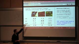
Andrej Karpathy covers linear classification for images using SVM hinge loss and softmax loss, then moves into optimization. He explains gradient descent, learning rates, and momentum, contrasting old hand-engineered features like SIFT with modern end-to-end learning.
Chapters
[Speaker:ANDREJ KARPATHY] So before we get— dive into some of the material today on loss functions and optimization, I wanted to go over some administrative things first. Just as a reminder, the first assignment is due on next Wednesday, so you have roughly 9 days left. And just as a warning, Monday is holidays, so there will be no class, no office hours. So plan out your time accordingly to make sure that you can complete the assignment in time. Of course, you also have some late days that you can use and allocate among your assignments as you see fit. Okay. So diving into the material, first I'd like to remind you where we are currently. Last time we looked at this problem of visual recognition, and specifically at image classification. And we were talking about the fact that this is actually a very difficult problem, right? So if you just consider the cross product of all the possible variations that we have to be robust to when we recognize any of these categories such as cat, it just seems like such an intractable, impossible problem. And not only do we know how to solve these problems now, but we can solve this problem for thousands of categories. And the state-of-the-art methods work almost at human accuracy or even slightly surpassing it in some of those classes. And it also runs nearly in real time on your phone. And so basically— and all of this also happened in the last 3 years. And also you'll be experts by the end of this class on all of this technology. So it's really cool and exciting. Okay. So that's the problem of image classification and visual recognition. We talked specifically about the data-driven approach and the fact that we can't just explicitly hardcode these classifiers, so we have to actually train them from data. And so we looked at the idea of having different— the training data having different validation splits where we test out our hyperparameters and a test set that you don't touch too much. We looked specifically at the example of the nearest neighbor classifier and so on, and the k-nearest neighbor classifier. And I talked about the CIFAR-10 dataset, which is our toe dataset that we play with during this class. Uh, then I introduced the idea of, uh, this approach that I termed parametric approach, uh, which is really that we're writing a function f from image directly to the raw 10 scores if you have 10 classes. And this parametric form, we assume to be linear first. So we just have f wx. And we talked about the interpretations of this linear classifier, the fact that you can interpret it as matching templates or that you can interpret it as these images being in a very high-dimensional space. and our linear classifiers are kind of going in and coloring this space by class scores, so to speak. And so by the end of the class, we got to this picture where we suppose we have a training example— training dataset of just 3 images here along the columns, and we have some classes, say 10 classes in CIFAR-10. And basically, this function f is assigning scores for every single one of these images with some particular setting of weights, which I've chosen randomly here. We get some scores out. And so some of these results are good and some of them are bad. So if you inspect the scores, for example, in the first image, you can see that the correct class, which is cat, got a score of 2.9, and that's kind of in the middle. So some, uh, some classes here received a higher score, which is not very good. Some classes received a much lower score, which is good for that particular image. Uh, the car was very well classified because the class score of car was much higher than all of the other ones, and the frog was not very well classified at all. Right? So we have this notion that for different weights, these different weights work better or worse on different images, and of course we're trying to find weights that give us scores that are consistent with all the ground truth labels, all the labels in the data. And so what we're going to do now is so far we've only eyeballed what I just described, like this is good or that's not so good and so on, but we have to actually give it— we have to actually quantify this notion. We have to say that this particular set of weights W is say like 12 bad. Or 1.5 bad or whatever. And then once we have this loss function, we're going to minimize it. So we're going to find w that gets us lowest loss, and we're going to look into that today. So we're going to look specifically into how we can define a loss function that measures this unhappiness, and then we're actually going to look at two different cases: a SVM cost and a softmax cost, or a cross-entropy cost. And then we're going to look into the process of optimization, which is how do you start off with these random weights and how do you actually find very, very good setting of weights efficiently. Okay. So I'm going to downsize this example so that we have a nice working example to work with. So suppose we only had 3 classes instead of, you know, tens of thousands, and we have these 3 images, and these are our scores for some set of Ws. And we're going to now try to write down exactly our unhappiness with this result. So the first loss we're going to look into is termed a multi-class SVM loss. This is a generalization of a binary support vector machine that you may have seen already in different classes. I think 229 covers it as well. And so the setup here is that, uh, we have the score function, right? So S is a vector of class scores. These are our S vectors, and there's a specific term here, loss equals to stuff. And I'm going to interpret this loss now for you so that— and we're going to see through a specific example, uh, into why this expression makes sense. Effectively, what the SVM loss is saying is that It's summing across all the incorrect examples. So all the, all the summing across all the incorrect scores, um, classes. So for every single example, we have that loss and it's summing across all the incorrect classes and it's comparing the score that the correct class received and the score that the incorrect class received, J minus S of Y_i, Y_i being the correct label, plus 1 and then that's maxed of 0. So what's going on here is we're comparing the difference in the scores, and this particular loss is saying that not only do I want the correct score to be higher than the incorrect score, but there's actually a safety margin that we're putting on. We're put— we're using a safety margin of exactly 1, and we're going to go into why 1 makes sense to use as opposed to some other hyperparameter that we have to choose there. And intuitively, you can look into notes for a much more rigorous derivation of exactly why that 1 doesn't matter, But intuitively, to think about this, the scores are kind of scale-free. Because I can scale my W, I can make it larger or smaller, and you're going to get larger or smaller scores. So really, there's this free parameter of these scores and how large or small they can be that is tied to how large your weights are in magnitude. And so these scores are kind of arbitrary. So using 1 is just an arbitrary choice to some extent. OK, so let's see specifically how this expression works with a concrete example. So here I'm going to evaluate that loss for the first example. So here we're computing, we're plugging in, uh, these scores. So we see that we're comparing the score we got for car, which is 5.1, minus 3.2, which is the correct class score, and then adding our safety margin of 1. And the max of 0 and that is really what it's doing is it's going to be clamping values at 0, right? So if we get a negative result, we're going to just clamp it at 0. So if you see for the second class score, the incorrect class of frog, -1.7. Subtract it from 3.2, add a safety margin, and we get -3.9. And then when you work this through, you get a loss of 2.9. So intuitively, what you can see here, the way this worked out is, intuitively, the cat score is 3.2. So according to the SVM loss, we, what we would like ideally is that the scores for all the incorrect classes are up to at most 2.2. But the car class actually had much higher, much higher score, 5.1. And this difference in what we would've liked, which is 2.2, and what actually happened, which is 5.1, is exactly this difference of 2.9, which is how bad of a score outcome this was. And, um, in the other case, in frog case, you can see that the frog score was quite a bit lower, below 2.2. And so the way that works out in the math is that you end up getting a negative number when you compare the scores, and then the max of 0 clamps it at 0, so you get a 0 loss contribution for that particular part, and you end up with a loss of 2.9, okay? So that's the loss for this first image. For the second image, we're going to again do the same thing, plug in the numbers. We're comparing the cat score to the car score. So we get, uh, 1.3 minus 4.9, add a safety margin, and the same for, uh, for the other class. So when you plug it in, you actually end up good with a loss of 0. And loss of 0 intuitively is because the car score here is— it is true that the car score is higher than all the other scores for that image. By at least 1, right? That's why we got 0 score— 0 loss, that is. So the constraint, uh, was satisfied, and so we get 0 loss. And in this frog case, we end up with a very bad loss because, of course, the frog class received a very low score, but the other classes received quite high score. So this adds up to an unhappiness of 10.9. And now, if we actually want to combine all of this into a single loss function, we're going to do the relatively intuitive, uh, transformation here where we just take the average across all the losses we obtain over the entire training set. And so we would say that the loss at the end when you average these numbers is 4.6. So this particular setting of W on this training data, uh, gives us some scores which we plug into the loss function and we given— we get an unhappiness of 4.6 with this result. Okay? So I'm now going to ask you a series of questions to kind of test your understanding a bit about how this works. Uh, I'll get into questions in a bit. Let me just pose my fir— my own questions first. Um, first of all, What if that sum over there, which is the sum over all the incorrect classes of j, what if that was instead sum over all the classes, not just the incorrect ones? So what if we allowed j to equal to yi? Why am I actually adding that small constraint in the sum over there? [Speaker] You're adding 1. [Speaker] Sorry, go ahead. [Speaker] You're adding the delta instead of the 1. [Speaker] Yes. So in fact, what would have happened is the reason that that's a j not equal to yi is if we allow j to equal to yi, then score of y_i cancels score of y_i. You end up with a 0, and really what you're doing is you're adding a constant of 1. So if that sum was over all the scores, then really we'd be just inflating the loss by a constant of 1. So that's why that's there. Um, second, what if we used a mean instead of a sum, right? So I'm summing up over all these constraints. What if I use the mean? Just like I'm using mean to actually, uh, average over all the losses for all the examples, what if I use the mean over the scores? The score constraints. Good. If you have too many classes, that would sort of dilute the loss. It's possible. So you're saying if there were too many classes, that would dilute the loss. Or like the— So you're right in that the absolute value of the loss would be lower. It would actually just be a constant factor. So it would be a constant factor, why? It would be the number of classes, you divide by the number of classes. That's right. Yeah. So is this— any of these choices kind of don't matter for your optimization, right? Uh, some of these choices matter. But yes, uh, so basically what you're pointing out is if we did actually do an average here, we'd be averaging over the number of classes here, but there's a constant number of classes, say 3 in this specific example. So that amounts to putting a constant of 1/3 in front of the loss. And since we're always in the end, so that would make the loss lower just like you pointed out. But in the end, what we're always interested in is we're going to minimize a W over that loss. So if you're— shifting your loss up by 1 or if you're scaling it with a constant, this actually doesn't change your solutions, right? You're still going to end up with the same optimal Ws. So these choices are kind of basically free parameters. It doesn't matter. So for convenience, I'm adding J not equal to Yi, and I'm not actually taking the mean, although it's the same thing. And the same also goes for us for whether or not we average or sum across the examples. Okay, next question. What if we instead used not the formulation over there, but a very similar looking formulation, but there's an additional squared at the end. So we're taking the difference between scores plus 1, this margin, and then we're squaring that. Do we obtain the same or different loss when you think— do we obtain the same or different loss in a sense that if you were to optimize this and find the best W, do we get the same result? Or not? Yes? [Speaker:AUDIENCE] Yeah, because you're thresholding it at 0. [INAUDIBLE] [Speaker:ANDREJ KARPATHY] So I like the fact that it's divided. You would, in fact, get a different loss. It's not as obvious to see, but one way to see it is that we're not just clearly scaling the loss up or down by a constant or shifting it by a constant. We're actually changing— the difference— we're changing the tradeoffs nonlinearly in terms of how the SVM, the support vector machine, is going to go there and trade off the different score margins in different examples. But it's not obvious to see. But basic— it's not very clear, but I wanted to illustrate that not all changes to this loss are completely a no-op. And the second formulation here is, in fact, called something we call a squared hinge loss instead of the one on top, which we call hinge loss. And you can use two different— it's kind of a hyperparameter which one you use. Most often you see the first formulation. That's what we use most of the time. But sometimes you can see datasets where the squared hinge loss ends up working better. So that's something you play with. That's really a hyperparameter, but its most often used, uh, form is the first one. Let's also think about the scale of this loss. Uh, what is the min and the max possible loss that you can achieve, uh, with the multiclass SVM on, on your entire dataset? What is the smallest value? 0. 0, good. What is the highest value? Infinite. Yeah, it's infinite, right. So basically, these scores could be arbitrarily terrible. So if your assigned score to the correct example is very, very small, then you're going to get your loss going to infinity. And one more question, which becomes kind of important when we start doing optimization. Usually when we actually optimize these loss functions, we start off with an initialization of W that are very small weights. So what ends up happening is that the scores at the very beginning of optimization are roughly near 0. All of these are like small numbers near 0. So what is the loss when all of these are near 0 in this particular case? The number of classes minus 1. That's right. Number of classes minus 1. So if all the scores are 0, then with this particular loss I put down here and by doing an average across this way, we would have achieved a loss of 2. Okay? So this is not very important. Where it's important is, for sanity checks when you're actually starting optimization and you're starting with very small numbers, w, and you print out your first loss as you're starting the optimization, and you want to make sure that you kind of understand the functional forms and that you can think through whether or not the number you get makes sense. So if I'm seeing 2 in this case, then I'm happy that the loss is maybe implemented correctly, but I'm not 100% sure. But certainly there's nothing wrong with it right away. So it's interesting to think about these. Um, let's see, I'm going to go more into this loss a tiny bit, but is there a question in terms of this slide right now? Go ahead. Yes, summing over j not equal to yi, wouldn't it be more efficient to not do that? So that you can take the matrix and sum over the whole matrix without asking to remove every, you know. Oh, yes. So the question is, and I was asked to repeat the questions, would it be not efficient to actually not have this ugly constraint j is not yi because it makes it more difficult to actually do these easy vectorized implementations of this loss implementation. So that actually predicts my next slide to some degree, so let me just go into that. So here's some NumPy code for how I would write out this loss function in vectorized NumPy code. So here we're evaluating Li in vectorized NumPy. We're getting a single example here. So x is a single column vector, y is an integer specifying the label, and w is our weight matrix. So what we do is we evaluate the scores, which is just, uh, w times x. Then we compute these margins, which is the difference between the scores we obtain and the correct score plus 1. So these are numbers between 0 and whatever. And then see this additional line, margins at y equals 0? Why is that there? [Speaker:AUDIENCE] It's the same as the current one. [Speaker:ANDREJ KARPATHY] Yeah, exactly. So basically I'm doing this efficient vectorized implementation, which goes to your point. And then I want to erase that margin. Margin there because I'm certain that margins at y currently is 1, and I don't want to inflate my score. And so I'll set that to 0. Sorry? Couldn't you just subtract 1 at the end? Yes, I suppose you could subtract 1 at the end as well. Very slightly faster cache-wise. That's right. So we can optimize this if we want, but we're not going to think about this too much. If you do in your assignment, that's very welcome for extra bonus points. And then we're summing up these margins, and so we get a loss in the end. OK? Going back to this slide, any more questions about this formulation? And by the way, this formulation, if you wanted to make it— if you actually write it down for just two classes, you'll see that it reduces to a binary support vector machine loss. OK, cool. So we'll see a different loss function soon, and then we're going to look at comparisons of them as well. But for now, actually, so at this point, what we have is We have this linear mapping to get scores, and then we have this loss function which I have now written out in its full form, where we have these differences between the scores, uh, plus 1, sum over the incorrect classes and the sum— and the average across all the examples, right? So that's the loss function right now. Now, I'd like to convince you that there's actually a bug with this loss function. In other words, if I'd like to use this loss on some dataset in practice, um, I might get some not very nice properties. OK, if this was the only thing I was using by itself. And it's not completely obvious to see exactly what the issue is, so I'll give you guys a hint. In particular, suppose that we found a W such that we're getting zero loss, OK, on some dataset. And now the question is, is this W unique? Or phrased in another way, can you give me a W that would be different but also definitely achieves a 0 loss? In the back? [Speaker:AUDIENCE] Yeah, we could scale it with a positive constant alpha or anything. [Speaker:ANDREJ KARPATHY] That's right. And so you're saying we can scale it by some constant alpha. And in particular, alpha must obey some constraint. [Speaker:AUDIENCE] And greater than 1. [Speaker:ANDREJ KARPATHY] You'd probably want it to be, yeah, greater than 1. Right. So basically what I can do is I can— if I change my weights and I make them larger and larger, all I would be doing is I'm just create— making the score difference larger and larger as I scale my W, right? Because of the linear loss form here. So basically, that's not a very desirable property because we have the— this entire subspace of W that is optimal, and all of them are, according to this loss function, completely the same. But intuitively, that's not like a very nice property to have. And so just to see this numerically, uh, to convince yourself that this is the case. I've taken this example where we achieved previously zero loss there before. And now suppose I multiply my w_i twice. I mean, this is a very simple math going on here, but basically I would be inflating all my scores by 2 times, and so their difference would also become just larger. So if all your score differences inside the max of 0 were already negative, then they're just going to become more and more negative. And so you end up with larger and larger negative values inside the maxes. And this just becomes 0 all the time. Go ahead. [Speaker:AUDIENCE] Why does alpha have to be larger than 1? [Speaker:ANDREJ KARPATHY] So the scaling factor would have to be larger than 1 because— let's see. [Speaker:AUDIENCE] There's a margin of 1, too? [Speaker:ANDREJ KARPATHY] Yeah, so there's that added margin of 1, which is complicating things. Yeah. OK. Another question? [Speaker:AUDIENCE] Yeah. Would the scaling apply to the bias part? So here I'm just— I guess I'm not assuming the bias for simplicity. But yeah, basically scores are wx plus b. So you're just— yeah, forget the bias and we're just scaling w by itself. Okay, cool. So the way to fix this is intuitively we have this entire subspace of w's and it all works the same according to this loss function. And what we'd like to do is we'd like to have a preference over some W's over others just based on intrinsic, you know, what, what do we desire of W to look like? Forget what the data is, just what, what are nice things to have about a W? And so this introduces the notion of regularization, which we're going to be appending to our loss function. So we have an additional term there, which is lambda times a regularization function of W. And the regularization function measures the niceness of your W, okay? And so we don't only want to fit the data, but we also want W to be nice. and we're going to see some, um, ways of, uh, framing that and exactly why they make sense. And intuitively what's going on is regularization is a way of trading off your training act— your training loss and your generalization loss on a test set. So intuitively regularization is a set of techniques where we're adding objectives to the loss which will be fighting with this guy. So this guy just wants to fit your training data and that guy wants W to look some particular way. And so they're fighting each other sometimes in your objective. Because we want to simultaneously achieve both of them. But it turns out that adding these regularization techniques, even if it makes your training error worse, so we're not correctly classifying all the examples, what you notice is that the test set performance ends up being better. And we'll see an example of why that might be. Actually, with the next— for now, I just wanted to point out in the next slide, but for now, I just wanted to point out that the most common form of regularization is the, what we call L2 regularization or weight decay. And really what we're doing is, uh, suppose W in this case is a 2D matrix. So I have two sums over K and L, the rows and columns. But really it's just all the element-wise Ws squared, and we're just putting them all into the loss, okay? So this, this particular regularization, it likes Ws to be, uh, 0, right? So when W is all 0, then regularization is happy. But of course W can't be all 0 because then you can't classify. So these guys will fight each other. There are different forms of regularization with different pros and cons. We'll go into some of them much later in the class. And I'd just like to say for now that basically L2 regularization is the most common form, and that's what you'll use quite often in this class as well. So now I'd like to convince you— I'd like to convince you that this is a reasonable thing to want out of a W, that its weights are small. So consider this very simple cooked-up example. To get the intuition. Suppose we have an example, um, where we are in 4-dimensional space where we're doing this classification and we have an input vector of just all 1s, x. And now suppose we have these two candidate weight matrices or weight— single weights, I suppose, right now. So one of them is 1, 0, 0, and the other is 0.25 everywhere. Since we have linear loss functions, you'll see that their effects are the same. So basically, the way we are evaluating score is by wx. So the dot product with x is identical for both of these. The scores would come out both of these. But regularization would strictly favor one of these over the other. Which one would the regularization cost favor? Even though their effects are the same, which one is better in terms of regularization? The second one, right? And so the regularization would tell you that even though they are achieving the same effects in terms of the data loss classification down the road, we actually significantly prefer the second one. What's better about this? The second one? Why is that a good idea to have? [INAUDIBLE] Sorry, can you repeat that? [INAUDIBLE] That's correct. So, well, that's one— that's the interpretation I like the most as well. It takes into account the most number of things in your x vector, right? So what this L2 regularization wants to do is it wants to spread out your w's, as much as possible so that you're taking into account all the input features or all the input pixels. It wants to use as many of those dimensions as it likes if it's achieving the same effect, intuitively speaking. And so that's better than just focusing on just one input dimension. It's just nice— it's something that often works in practice, basically, just the way things are— datasets are arranged and the properties that they usually have statistically. OK? Any questions about this? So regularization, good idea? Everyone is sold? OK, great. So basically, our losses will always have this form, where we have the data loss, and then we'll also have a regularization. It's a very common thing to have in practice. OK. I'm now going to go into the second classifier, the softmax classifier. And we'll see some differences between the support vector machine and this softmax classifier. In practice, these are kind of like these two choices that you can have, either SVM or softmax. The most two commonly used linear classifiers. Often you'll see that softmax classifier is preferred, and I'm not exactly sure why because usually they end up working about the same. And I'd just like to mention that this is also sometimes called multinomial logistic regression. So if you're familiar with logistic regression, this is just a generalization of it into multiple dimensions, or in this case, multiple classes, not just two. Was there a question over there or? [Speaker] Yeah, so I was wondering on a higher level why you would want to —regularization? Is it to choose which weight is better given that they have the same loss? Yes, so the question is, why do we want to use regularization, basically? So I don't think I sold it very well. Suppose you have this entire subspace of weights that is all achieving the same effects. We'd like to pick between them in some way. And I think what I'm arguing for is that wanting low W's is a reasonable way to pick among them, and the L2 regularization will favor diffuse W's like in this case here. And one of the intuitive ways in which I can try to pitch why this is a good idea is that diffuse weights basically— see this W1 is completely ignoring your inputs 2, 3, and 4, but W2 is using all of the inputs, right, because the weights are more diffuse. And so intuitively this just ends up usually working better at test time because more evidence is being accumulated into your decisions instead of just one single evidence, one single feature. And to follow up, so you add it as a part of the sum, right? That's right. And so in this case, W2 would have a higher value than W1. That's right. It would have a higher loss. That's right. So the idea here is that these two, W1 and W2, they're achieving the same effect. So this data loss, suppose that that's basically— it doesn't care between the two. But the regularization expresses preference for them. And since we have it in the objective, and we're going to end up optimizing over this loss function, so we're going to find a W that simultaneously accomplishes both of those. And so we end up with W that not only classifies correctly, but we also have this added preference that actually we want it to be diffuse as much as possible. Make sense? Awesome. Go ahead. [Speaker:AUDIENCE] If we want that to be the case, why would we use L1 originally? Can we solve this in those tools too? [Speaker:ANDREJ KARPATHY] Yes, so in this particular example, L1 would also be indifferent. L1 has some nice properties, which I don't want to go into right now. We might cover it later. L1 has some properties like sparsity-inducing properties where if you end up having L1s in your objectives, you'll find that lots of w's will end up being exactly 0. For reasons that we might go into later. And that sometimes is like a feature selection almost. And so L1 is another alternative that we might go into a bit more later. Go ahead. [Speaker:AUDIENCE] Yeah, doesn't the W1 on the other slide have the nice property? Isn't it good that you're ignoring some of the features if they're not actually giving you a better loss? [Speaker:ANDREJ KARPATHY] Yeah, so the question is— Yeah. So you're pointing out that isn't it maybe a good thing that we're ignoring features and just using one of them? Yeah. So there's many technical reasons why regularization is a good idea. I wanted to give you just basic intuition. So maybe I failed at that. But yeah, I think that's a fair point. Yeah. I'm not sure if I have a good return. I would have to— go ahead. Couldn't you say that epsilon 0, 0, 0 would do the exact same thing as w1, or like with epsilon being a really small number, so that that vector would do the exact same thing but would also have small, much smaller regularization? So you want to consider a different w, and you want it to look slightly different from these two? I'm just saying like the previous question was like, isn't it good that we're ignoring some values? So why would w2 be— Yeah, isn't that a feature, not a bug, that we're ignoring some inputs? So I was saying that you could just have like 0.001, 0, 0, 0 as another w vector that would do exactly the same thing as w1. In terms of its decisions, but it would— I don't know, just throwing that out. I see. OK. Thanks. Yeah. I didn't want to dive too much into this. There's actually an entire literature of regularization and looking at the test error and actually writing theorems and learning theory. And you saw some of that in 229. And there are some results on why regularization is a good case in those areas. I don't think I want to go into that. And it's also beyond the scope of this class. So for this class, just ultra-regularization will make your test error better. [LAUGHTER] OK. So I'm going to go into Softmax classifier now, which is this generalization of logistic regression. So the way this will work is this is just a different functional form for how loss is specified on top of these scores. So in particular, there's this interpretation that Softmax classifier puts on top of these scores. These are not just some arbitrary scores and we want some margins to be met, but we have specific interpretation that is maybe more principled, uh, kind of from a probabilistic point of view where we actually interpret these scores not just as these things that mean margins, but these are actually the un-normalized log probabilities that are assigned to different classes. Okay? So we're going to go into exactly what this means in a bit. So these are un-normalized log probabilities of all the Ys given the image. So in other words, we're assuming that if the scores are unnormalized log probabilities, then the way to get probabilities of different classes like class K is that we take these— the score, we exponentiate all of them to get the, um, the unnormalized probabilities and we normalize them to get the normalized probabilities. So we divide by the sum over all the, um, exponentiated scores. And that's how we actually get this expression for a probability of a class given the image. And so this function here is called the softmax function, if you'll— if you see it somewhere. Uh, it's the e to the, um, the element you're currently interested in divided by the sum over all exponentiated scores, okay? And so the way this will work basically is if we're in this probabilistic framework where we are looking at— we're deciding that this is the probability of different classes, then it makes sense in terms of what you usually want to do in this setting. We have probability over different classes, one of these is correct. So we want to just maximize the log likelihood of, um, for the loss function. And sorry, we want to maximize the log likelihood of the true class. And since we're writing a loss function, we want to minimize the negative log likelihood of the true class. Okay? So you end up with a series of expressions here. Really, our loss function is we want the log likelihood of the correct class to be high, so negative of it want to be low. And the log likelihood is softmax function of your scores. Let's look at a specific example to make this more clear. Um, okay, and here I've actually, like, subbed in that expression so that this is the loss, negative log of that expression. Let's look at how this expression works, and I think it will give you a better intuition of exactly what this is doing, why it's— what it's computing. So suppose here we have these scores that came out from our neural network or from our linear classifier. And these are the un-normalized log probabilities. So as I mentioned, we want to exponentiate them first because under this interpretation, that gives us the normalized probabilities. And now probabilities always sum to 1, so we have to divide by the sum of all of these. So we add up these guys and we divide to actually get probabilities out. So under this interpretation, we've carried out the set of transformations, and what this is saying is that in this interpretation, the probability assigned to this image of being a cat is 13%, car is 87%, and frog is very unlikely, 0%. So these are the probabilities. And now normally in this setting, you want to maximize the log probability, because it turns out that maximizing just the raw probability is not as nice mathematically. So normally you see maximizing log probabilities. And then so we want to minimize the negative log probability. So the correct class here is cat, which is only having 13% chance under this interpretation. So negative log of 0.13 gives us 0.89. And so that's the final loss that we would achieve for this class here under this interpretation of a softmax classifier. So 0.89 for softmax. OK? So let's go over some examples. Let's go over some questions now related to this to try to interpret exactly how this works. Uh, what is the min and the max possible loss with this loss function? So that's the loss function. What is the smallest value and the highest value? So I'll give you a chance to think about this. What is the smallest value that we can achieve? 0. 0. And how would that happen? Log of the percent. Okay, good. So if your correct class is getting probability of 1, we're— we have a 1 which we're plugging into the log and we're getting negative log of 1 which is 0. And the highest possible loss? Infinite. So just as with SVM, we're getting the same. 0 is minimum, and infinite is maximum. So infinite loss would be achieved if you end up giving your cat score very tiny probability. And then log of 0 gives you negative infinity. So negative that is just infinite. So yeah, so the same bounds as SVM. And also this question, normally when we initialize W with roughly small weights, we end up with all the scores that are nearly 0. What ends up being the loss in this case if you're doing sanity checks at the beginning of your optimization? What do you expect to see as your first loss? Yeah, go ahead. [Speaker:AUDIENCE] Log of 1 over number of classes, negative. Yeah, that's right. So, uh, it's negative log of 1 over number of classes. So you'd basically be getting all zeros here, you get all ones here, and so here is 1 over the number of classes, and then negative log of that ends up being your final loss. So actually for myself, whenever I, uh, run optimization, I sometimes take note of my number of classes and I evaluate negative log of 1 over the number of classes, and I'm trying to see what is the— my first beginning loss that I expect. And so when I start the optimization, I make sure that I'm getting roughly that. Otherwise, I know something's maybe slightly off. I expect to get something on that order. Moreover, as I'm optimizing, I expect that I go from that to 0. And if I'm seeing negative numbers, then I know from the functional form that something very strange is going on, right? Because you never actually expect to get negative numbers out of this. So that's the softmax loss. I'll show you one more slide, and I'll take some questions. Just to reiterate the difference between them and really what they look like is we have the score function, which gives us wx times b. We get our scores vector. And now the difference is just how they interpret what these scores coming out from this, um, f function is. So either it's just random scores, no interpretation whatsoever. We just want the lar— larger score, the correct score to be some margin above the incorrect scores. Or we interpret it to be these un-normalized log probabilities. And then in this framework, we first want to get the probabilities, and then we want to maximize the probability of the correct classes or the log of them. And so that ends up giving us the loss function for softmax. So they start off with the same way, but they just happen to get a different slight result. We'll go into exactly what the differences of them are in a bit. There are questions for now? So, uh, these don't take significantly different times to— amounts of time to calculate, right? Uh, that's correct. So they, they take about the same time to calculate for sure, especially once you have a ConvNet. Your classifier is near instantaneous to evaluate. Most of the work is done in doing all the convolutions. And so we'll see that the classifier, and especially the loss, is roughly the same. Of course, softmax involves some exp and so on. So these operations are slightly more expensive perhaps. But usually it completely washes away compared to everything else you're worried about, which is all the convolutions over the image. Go ahead. [Speaker:AUDIENCE] What do we take, uh, low function even if the final value tells us the probability of value? Like if 0.631 is the highest number, that is more likely to be an answer? Sorry, I didn't catch your question fully. Why do we have to take log function at the end? Why do we want to maximize log probabilities instead of probabilities directly? It turns out when you— So this is partly covered in 229 when you do logistic regressions and so on. If you just want to maximize probability, it would, it would be the exact same problem because log is a monotonic function. And so maximizing the probability and maximizing the log probability give you the identical result. But in terms of the math, everything comes out much nicer looking when you actually put a log there. But it's the exact same optimization problem. Okay, cool. Let's look at some interpretations of these two and exactly how they differ. So softmax versus SVM and trying to give you an idea about one property that actually is quite different between the two. Um, so they have these two different functional forms. And now assume that we have these three examples, all three examples, and suppose there are three classes, three different examples, and these are the scores of these examples. And for every one of these examples, the first class here is the correct class. So 10 is the correct class score, and the other scores are, these guys, either the first one, second, or third one. And now, uh, just think about what these losses tell you about how desirable these outcomes are in terms of that W. Um, and in particular, one way to think about it, for example, is suppose I take this data point, the third one, 10, -100, -100, and suppose I jiggle it, like I, I move it around a bit in my input space. What is happening to the losses as I do that? [Speaker:AUDIENCE] Like increases and decreases depending on what direction you move in. [Speaker:ANDREJ KARPATHY] OK. So they increase and decrease as I wiggle this data point around. Do they both increase or decrease for the third data point, for example? [Speaker:AUDIENCE] No. SVM remains the same. [Speaker:ANDREJ KARPATHY] SVM remains the same, correct. And why is that? It's because the margin was met by a huge amount So there's this added robustness. When I take this data point and I shake it around, the SVM is already very happy because the margins were met by, you know, we desire a margin of 1, and here we have a margin of 109. So basically there's a huge amount of margin. The SVM doesn't express a preference over these examples where the scores come out very negative. Then the SVM adds no additional preference over, do I want these to be -20 or -100 or -1,000? The SVM won't care. But the softmax could always see— you would always get an improvement for softmax, right? So softmax function expresses preference for— it wants these to be negative 200 or 500 or 1,000. All of them would give you better loss, right? But the SVM at this point doesn't care. And for the other examples, I don't know if it's as— I mean, that's one clear distinction, right? So the SVM has this added robustness to— it wants this margin to be met, but beyond that, it doesn't micromanage your scores. Where softmax will always want these scores to be, you know, everything here, nothing there. And so, um, that's one kind of a very clear difference between the two. That was their question? Go ahead. Yeah. Uh, maybe I missed this, but is there a— is the margin that 1, is that a hyperparameter? Is that something that gets changed? Uh, yes. So the margin of 1, I mentioned very briefly that that's not a hyperparameter. You can fix it to be 1. The reason for that is that these scores, the absolute values of those scores are kind of— they don't really matter. Because my w, I can make it larger or smaller, and I can achieve different size scores. And so 1 turns out to work better. And in the notes, I have a longer derivation where I go into details exactly why 1 is safe to choose. So refer to that. But I didn't want to spend time on it in the lecture. [Speaker:AUDIENCE] So the notes do justify not using 0? [Speaker:ANDREJ KARPATHY] Oh, so 0 would be— if you wanted to use 0, that would be trouble. You can use any positive number, and that would give you an SVM. If you use 0, that would look different. So for example, this added constant there, one property it gives you when you actually go through the mathematical analysis, like say in the SVM in CS229, is you'll see that it achieves this max margin property. Where the SVM will find the best margin when you actually have a plus constant there combined with the L2 regularization on the weights. So you want very small weights that meet a specific margin, and SVM will give you this very nice max margin property that I didn't really go into in this lecture right now. But basically, you do want the positive number there, otherwise things would break. Go ahead. Is there a reason we're interpreting that exponential value as probabilities? Is there a special reason we call it probabilities other than that it's not negative? Yeah, is there— so you're saying we're taking this exponential of these numbers that are real numbers, and we're interpreting them as probabilities. We're kind of free to— so with this, you're getting these scores out, and it's up to you to to endow them with interpretation, right? We can have different losses. In this specific case I showed you, multiclass SVM, there's in fact multiple versions of a multiclass SVM. You can fiddle around with exactly the loss expression. And one of the interpretations we can put on this course is that there are these unnormalized log probabilities. They can't be normalized because they just can't— we have to normalize them explicitly because there's no constraint that the output of your function will be normalized. And they can't be probabilities because you're outputting just these real numbers that can be positive or negative. So we interpret them as log probabilities, and that requires us to exponentiate them. It's a very bad explanation of it, but anyways. Go ahead. Just add on to what you just said. So that's actually pretty similar to Boltzmann statistics. If you interpret score as energy, then that's exactly the probability that energy is being occupied. Yeah, that's right. So there are really cool connections to physics and how they actually think about loss functions. For them, energy and loss is kind of an equivalent as well. Good. We're talking about the SVM versus softmax. Once it goes beyond a certain margin, of 2 or 3 and you're going to exponentiate it, the difference you will get in softmax is going to be vanishingly small. So you're talking about, so say for example, in this case? Yeah. Very good. And now you're arguing about, say, this one? Yeah. OK. If 100 minus 100 goes to minus 110, it's still not going to really change your probabilities a lot. That's right. So what you're saying, I think, if I understand correctly, is the softmax would already look at this and give 0 probabilities here and 1 here, right? So you're saying if I jiggle this around, nothing's changing. I think the difference is the loss would definitely change for softmax, even though it wouldn't change a lot, but it would definitely change. So softmax still expresses preference, whereas SVM gets you identically 0, right? My question is about the magnitude of that preference. Isn't it just not very big? Uh, yeah. Yeah, so the preference wouldn't be very big, but there definitely is preference. But in practice, basically, this distinction— the intuition I'm trying to give you is that the SVM has a very local part of the space in which you're classifying that it cares about. And beyond it, it's invariant. And a softmax kind of is a function of the full data cloud. It cares about all the points in your data cloud, not just— you know, there's like a small class here that you're trying to separate out from everything else. A softmax will kind of consider the full data cloud when it's fitting your plane, and SVM will just want to separate out that tiny piece from the immediate part of the data cloud, something like that. In practice, when you actually run these, they kind of give nearly identical results almost always. So really what I'm trying to— I'm not trying to pitch one or the other. I'm just trying to give you this notion that you're in charge of the loss function. You get some scores out, and you can write down nearly any mathematical expression as long as it's differentiable into what you want your scores to be like. And there are different ways of actually formulating this. And I've shown you two examples that are common to see in practice. But in practice— and we can put down any losses for what you want your scores to be. And that's a very nice feature because we can optimize over all of it. OK, let me show you an interactive web demo at this point. Jeffrey. All right, let's see this. So this is an interactive demo on our class page. You can find it at this URL. I wrote it last year, and I have to show it to all of you guys to justify spending one day on developing all this. OK. But so I'm not sure— last year not too many people looked at this, so OK. But basically, this is one day of my life. You should all look at this. So what we have here is a two-dimensional problem with three classes. And I'm showing here three classes, each has three examples over here in two dimensions. And I'm showing the three classifiers here as the level set. So for example, the red classifier is— has scores of 0 along the line. And then I'm showing the arrows in which the scores increase, right? Here's our W matrix. So as you recall, this W matrix, the rows of that W matrix are the different classifiers. So we have the blue classifier, red— green classifier, and red classifier. And we have both the weights for both the x and the y component, and also the biases. And then here we have the datasets. So we have the x and the y coordinate of all the data points, their correct label, and the scores, as well as the loss achieved by all those data points right now with this setting of w. And so you can see that I'm taking the mean over all the loss. So right now our data loss is 2.77, regularization loss for this w is 3.5, And so our total loss is 6.27, okay? And so basically you can fiddle around with this. So let's see. So as I change my w, you can see that here I'm making my w— one of the w's bigger, and you can see what that does in, in there, or the bias. You can see that the bias basically shifts these hyperplanes. Um, okay. And then what we can do is we can— what we're going towards, this is kind of a preview of what's going to happen. We're getting the loss here. And then we're going to do backpropagation, which is giving us the gradient over how we want to adjust these W's in order to make the loss smaller. And so what we're going to do is this repeated updates where we start off with this W, but now I can improve, uh, I can improve this set of W's. So when I do a parameter update, this is actually using these gradients which are shown here in red, and it's actually making a tiny change to every single parameter according to this gradient, right? right? So as I do parameter update, you can see that the loss here is decreasing, especially the total loss here. So the loss just keeps getting better and better as I do parameter update. So this is the process of optimization that we're going to go into in a bit. So I can also start a repeated update, and then basically we keep improving this W over and over until our loss— it started off with roughly 3 or something like that. So now our mean loss over the data is 0.1 or something like that, and we're correctly classifying all these, all these points here. Um, so I can also, uh, randomize, randomize W, so it just kind of knocks it off, and then this always converges to the exact same point through the process of optimization. And, um, you can play here with the regularization as well. You have different forms of a loss. So the one I've shown you right now is the Weston-Watkins SVM formulation. There's a few more SVM formulations And there's also softmax here. And you'll see that when I switch to softmax loss, our losses look different, and— but the solution ends up being roughly the same. So when I switch back to NSVM, you know, the hyperplanes move around a tiny bit, but really it's mostly the same. And so anyways, so this is the step size. So this is how much— how big of steps are we making when we get the gradient on how to improve things. So randomized parameters, we usually start with a very big step size. These things are jiggling, trying to separate out these data points. And then over time, what we're going to be doing in optimization is we're going to decrease our update size. And this thing will just slowly converge in on the parameters that we want in the end. And so you guys can play with this, and you can see how these cores jiggle around and what the loss is. And if I stop a repeated update— wait, wait, here it is. You can also drag these points, but I think on the Mac it doesn't work. So when I try to drag this point, it disappears. So— [LAUGHTER] But it works on a desktop. So I don't want to go in and figure out exactly what happened there. But— so you can play with this. OK. Cool. So I'm going to go into the process of optimization now. Just to give you a sense of what this looks like. So we have this f function. We have these two formulations that I've shown you. And the full loss is achieved as the mean loss over data plus regularization. This is one other diagram to show you how— what this looks like. I don't think it's a very good diagram. And there's something confusing about it that I can't remember from last year. But basically, you have this data x and y. Images and your labels, and there's W, and we're computing the scores and getting the loss, and the regularization loss is only a function of the weights, not of the data. And basically what we want to do now is we don't have control over the dataset, right? That's given to us. But we have control over that W, and as we change that W, the loss will be different. So for any W you give me, I can compute the loss, and that loss is linked to how well we're classifying all of our examples. So wanting a low loss means we're classifying them very, very well on the training data. And then we're crossing our fingers that that also works on some test data that we haven't seen. So here's one strategy for optimization. It's a random search. So because we can evaluate loss for any arbitrary W, what I can afford to do— and I'm not sure if— I don't want to go through this in full detail. But effectively, I randomly sample Ws, and I can check their loss. and I can just keep track of the W that works best, okay? So that's an amazing process of optimization of guess and check. And it turns out if you do this, I think I tried 1,000 times. If you do this 1,000 times and you take the best W you found at random and you run it on your CIFAR-10 data, test data, you end up with about 15.5% accuracy. And since there are 10 classes in CIFAR, the mean, um, the baseline is at 10%. That's your chance performance. So 15.5, there's some signal actually in that W. And so state of the art is at 95, which is a ConvNet. So we have some gap to close over the next 2 weeks or so. So this is— so don't use this just because it's on the slides. One interpretation of exactly what this looks like, this process of optimization, is that we have this loss landscape, right? This loss landscape is in this high-dimensional W space. So here we— I guess if you're in 3D and your loss is the height, then you only have 2 Ws in this case. And you're here and you're blindfolded. That's your current W. You can't see where the valleys are, but you're trying to find low loss. And so you're blindfolded and you have an altitude meter. And so you can tell what your loss is at any single point. And you're trying to get to the bottom of the valley, right? And so that's really the process of— optimization. And what we've shown you— what I've shown you so far is this random optimization where you teleport around and you just check your altitude, right? So not the best idea. So what we're going to do instead is we're going to use what I refer to already as a gradient. Or really, we're just computing the slope across in every single direction. So I'm trying to compute the slope, and then I'm going to go downhill, OK? So we're following the slope. I'm not going to go into too much detail on this, but basically there's an expression for the gradient, which is defined like that. There's a derivative, calculus 101 definition. In multiple dimensions, if you have a vector of derivatives, that's referred to as the gradient, right? So because we have multiple dimensions, multiple Ws, we have a gradient vector, okay? So this is the expression, and in fact, we can numerically evaluate this expression. Expression before I go into the analytic solution. I'll just show you what that would look like to evaluate a gradient at some w. So suppose we have some current w, and we're getting some loss. What we want to do now is we want to get an idea about the slope at this point. So we're going to basically look at this formula, and we're just going to evaluate it. So I'm going to go in the first dimension, and I'm going— and really what this formula is telling you to do is evaluate x plus— your altitude at x h, subtract it from f(x), and divide by h. What that corresponds to is me being on this landscape, taking a small step in some direction, and looking whether or not my foot went up or down, right? That's what the gradient is telling me. So suppose I took a small step and the loss there is 1.25. Then I can use that formula with a finite difference approximation where I've used a small h to actually derive that the gradient here is -2.5. The slope the slope is downwards. So I took a step, the loss decreased, so this is sloping downwards in terms of the loss function. So -2.5 in that particular dimension. So now I can do this for every single dimension independently, right? So I go into the second dimension, I add a small amount, so I step in a different direction, I look at what happened to the loss, I use that formula, and it's telling me that the gradient, the slope, is 0.6. And I can do that in the third dimension, and I get the gradient there, okay? So what I'm referring to here is I'm basically evaluating the num— the numerical gradient, which is using this finite difference approximation where for every single dimension independently, I can take a small step, I can evaluate the loss, and that tells me the slope. Is it going upwards or downwards for every single one of these parameters? And so, uh, this is, um, evaluating numerical gradient. The way this would look like is, uh, Python function here. It looks ugly because it turns out it's slightly tricky to iterate over all the W's. But basically, we're just looking at f(x h) comparing to f(x) and dividing by h, and we're getting the gradient. Now, the problem with this is if you want to use the numerical gradient, then of course, we have to do this for every single dimension to get a sense of what the gradient is in every single dimension. And right, um, when you have a ConvNet, you have hundreds of millions of parameters, right? So we can't afford to actually check the loss in hundreds of millions of parameters before we do a single step. So this approach where we would try to evaluate the gradient numerically is— first of all, it's approximate because we're using finite difference approximations. But second, it's also extremely slow because I need to do a million checks of the loss function on my ConvNet before I know what the gradient is and I can take a parameter update. So very slow, approximate. Turns out that this is also silly, right? Because the loss is a function of w as we've written it out. And really what we want is we want the gradient of the loss function with respect to w. And luckily, we can just write that down thanks to these guys. Do you actually know who those guys are, by the way? Newton and Leibniz. Newton and Leibniz, that's right. Do you know which is which? Because they look the same. They're just— yeah, they look remarkably similar. But basically, Newton and Leibniz It's sort of two inventors of calculus. There's actually controversy over who really invented calculus. And these guys fought each other over it. But basically calculus is this powerful hammer. And so what we can do is instead of doing the silly thing where we're evaluating numerical gradient, we can actually use calculus and we can write down an expression for what the gradient is of that loss function in the weight space. So basically instead of fumbling around and doing this, is it going up or is it going down by checking the loss? I just have an expression where I take the gradient of this, and I can simply evaluate what that entire vector is. So that's the only way that you can actually run this in practice, right? We can just have an expression for here's the gradient, we could do a step, and so on. So in summary, basically numerical gradient approximate slow, but very easy to write because you're just doing this very simple process for any arbitrary loss function. I can get the gradient vector. For analytic gradient, which is you actually do calculus, it's exact, no finite approximations. It's very fast, but it's error-prone because you actually have to do math, right? So in practice, what you see is we always use analytic gradient. We do the calculus. We figure out what the gradient should be. But then you always check your implementation using a numerical gradient check, as it's referred to. So I will do all my calculus. I figure out what the loss function should be. I write an expression for the gradient. I evaluate it in my code. So I get an analytic gradient. And then I also evaluate a numerical gradient on the side. And that takes a while, but you enumerate your— you evaluate your numerical gradient. And you make sure that those two are the same. And then we say that you pass the gradient check. OK, so that's what you see in practice. Whenever you try to develop a new module for your neural network, you write out its loss. You write the backward pass for it that computes the gradient. And then you have to make sure to gradient check it just to make sure that your calculus is correct. And then I've already referred to this process of optimization, which we saw nicely in the web demo, where we have this loop when we optimize, where we simply evaluate the gradient on your loss function. And then knowing the gradient, we can perform a parameter update where we change this W by a tiny amount. In particular, we want to update with the negative step size times the gradient. The negative is there because the gradient tells you the direction of the greatest increase. It tells you which way the loss is increasing, and we want to minimize it, which is where the negative is coming from. We have to go in the negative gradient direction. Step size here is a hyperparameter that will cause you a huge amount of headaches. Step size or learning rate, this is the most critical parameter to basically worry about, uh, that, uh, really there's two that you have to worry about the most, the step size or learning rate, And there's the weight regularization strength lambda that we saw already. Those two parameters are really the two largest headaches. And that's usually what we cross-validate over. Was there a question in the back, by the way? Yeah. I was just going to ask, is that weight gradient vector a unit vector, or— It's not. That gradient is just gradient. It tells you the slope in every single direction. And then we just take a step-size step of it. So the process of optimization in this weight space is you're somewhere in your W, you get your gradient, and you march some amount in the direction of the gradient. Um, but you don't know how much, so that's the step size. And you saw that when I increased the step size in the demo, things were jiggling— jittering around quite a lot, right? There was a lot of energy in the system. That's because I was taking huge jumps all over this basin. So here the loss function is minimal at the blue part there, and it's high in the red parts. So we want to get to the, uh, lowest part of the basin. This is actually what the loss function looks like for an SVM or for logistic regression. These are convex problems. So it's really just a bowl, and we're trying to get to the bottom of it. But this bowl is like 30,000-dimensional, so that's why it takes a while. Um, okay. So we take a step, and we reevaluate the gradient and repeat this over and over. In practice, uh, there's this additional, uh, part I wanted to mention where we don't actually evaluate the loss for the entire training dataset. In fact, what we do is we only use what's called a mini-batch gradient descent, where we have this entire dataset, but we sample batches from it. So we sample, say, like, say, 32 examples out of my training data. I evaluate the loss and the gradient on this batch of 32, and then I do my parameter update, and I keep doing this over and over again. And basically what ends up happening is if you only sample very few data points from your training data, then your estimate of the, Approximate gradient, of course, over the entire training set is kind of noisy because you're only estimating it based on a small subset of your data, but it allows you to step more. So you can do more steps with approximate gradient, or you can do few steps with exact gradient. And in practice, what ends up, um, working better is if you use mini-batch. And, uh, it's much more efficient, of course, and, uh, it's impractical to actually do full batch gradient descent. So common mini-batch sizes: 32, 64, 128, 256. This is not usually a hyperparameter we worry about too much. You usually set it based on whatever fits on your GPU. We're going to be talking about GPUs in a bit, but they have finite amount of memory, say about like 6 gigabytes or 12 gigabytes if you have a good GPU. And you usually choose a batch size such that a small mini-batch of examples fits in your memory. So that's how usually that's determined. It's not a hyperparameter that actually matters a lot in an optimization sense. Go ahead. [Speaker:AUDIENCE] If you wanted to use— If you use momentum on the step size, could you still do it with the mini-batch update? Yeah, for sure. And we're going to get to momentum in a bit. But if you wanted to use momentum, then yeah, this is just fine. We always use mini-batch gradient descent with momentum. Very common to do. So just to give you an idea about what this looks like in practice, if I'm running optimization over time and I'm looking at the loss evaluated on just a small mini-batch of data, and you can see that basically my loss goes down over time on these mini-batches from the training data. So as I'm optimizing, I'm going downhill. Now, of course, if I was doing full batch gradient descent, so this was not just mini-batches sampled from the data, you wouldn't expect as much noise. You just expect this to be a line that just goes down. But because we use mini-batches, you get this noise in there because some mini-batches are better than others. But over time, they kind of all go down over time. Is there a question? [Speaker:AUDIENCE] I'm just trying to figure out if you are Shouldn't the graph look like it decreases greatly in the beginning and sort of— [INAUDIBLE] Yeah, so you're wondering about the shape of this loss function. You're used to maybe seeing more rapid improvement quicker. These loss functions come in different shapes, sizes. So it really depends. It's not necessarily the case that a loss function must look very sharp in the beginning, although sometimes they do. They have different shapes. For example, it also matters on your initialization. If I'm careful with my initialization, I would expect less of a jump. But if I initialize very incorrectly, then you would expect that that's going to be fixed very early on in the optimization. We're going to get to some of those parts, I think, much later. I also wanted to show you a plot of the effects of learning rate on your loss function. And this learning rate is the step size. Basically, if you have very high learning rates or step sizes, you start thrashing around in your W space. And so either you don't converge or you explode. If you have a very low learning rate, then you're barely doing any updates at all. So it takes a very long time to actually converge. And if you have a high learning rate, sometimes you can basically get kind of stuck in a bad position of a loss. So these loss functions kind of— you need to get down to the minimum. So if you have too much energy and you're stepping too quickly, then you don't have— you don't allow your problem to kind of settle in on the smaller local minima in your objective. In general, when you talk about neural networks and optimization, you'll see a lot of hand waving because that's the only way we communicate about these losses and basins. So just imagine like a big basin of loss, and there are these like smaller pockets of smaller loss. And so if you're thrashing around, then you can't settle in on the smaller loss parts and converge further. So that's why learning rate is no good. And so you need to find the correct learning rate. Which will cause you a lot of headaches. And what people do most of the time is sometimes you start off with a high learning rate so you get some benefits, and then you decay it over time. So you start off with high, and then we decay this learning rate over time as we're settling in on a good solution. And, um, I also wanted to point out— we'll go into this in much more detail— but the way I'm doing the update here, which is how do you use the gradients to actually modify your w, that's called an update. Parameter update, there are many different forms of doing it. This is the simplest way, which we refer to as just SGD, simplest stochastic gradient descent. But there are many formulas such as momentum that was already mentioned. In momentum, you basically imagine, as you're doing this optimization, you imagine keeping track of this velocity. So as I'm stepping, I'm also keeping track of my velocity. So if I keep seeing a positive gradient in some direction, I will accumulate velocity in that direction. So I don't need— So I'm going to go faster in that direction. And so there are several formulas. We'll look at them shortly in the class, but AdaGrad, RMSProp, Adam, all commonly used. So just to show you effect of different— what these look like, these different choices and what they might do in your loss function, this is a figure from Alec. So here we have a loss function, and these are the level curves. And we start off optimization over there, and we're trying to get to the basin. And different update formulas will give you better or worse convergence in different problems. So you can see, for example, this momentum in green, it built up momentum as it went down, and then it overshot, and then it kind of goes back. And this SGD takes forever to converge in red. That's what I presented you so far. So SGD takes forever to converge, and there are different ways of actually performing this parameter update that are more or less efficient in the case of optimization. Yeah. So we'll see much more of this soon. I also wanted to mention at this point, slightly shifting gears, I wanted to go slightly into— I've explained now basically linear classification. We know how to set up the problem. We know there are different loss functions. We know how to optimize them. So we can kind of do linear classifiers at this point in the class. I wanted to mention that I want to give you a sense of what computer vision looked like before ConvNets came about so that you have a bit of historical perspectives. Because we used linear classifiers all the time, but of course you don't use linear classifiers on the raw original image because that's a pixel. You don't want to put linear classifiers on pixels. We saw all the problems with it, like you have to cover all the modes and so on. So what people used to do is they used to compute all these different feature types out of images, and then you compute different descriptors and different feature types, and you get these statistical summaries of what the image looks like, what the frequencies are like, and so on. and then we concatenated all those into large vectors, and then we piped those into linear classifiers. So different feature types, all of them concatenated, and then that went into linear classifiers. That was usually the pipeline. So just to give you an idea of really what these feature types were like, one very simple feature type you might imagine is just a color histogram. So I go over all the pixels in the image, and I bin them into, say, uh, how many bins are there for different colors depending on the hue of the color. And so you can imagine this is kind of like one statistical summary of what's in the image. It's just number of colors in each bin. So this would become one of my features that I would eventually be concatenating with many different feature types. Another kind of— and so basically the classifier, if you think about it, the linear classifier can use these features to actually perform the classification because the linear classifier can like or dislike seeing lots of different colors in the image with positive or negative weights. Very common features also included things like what we call sift-and-hog features. Basically, these were— you go in local neighborhoods in the image and you look at whether or not there are lots of edges of different orientations. So are there lots of horizontal edges or vertical edges? We make up histograms over that. And so then you end up with just this summary of what kinds of edges are where in the image, and you concatenate all those together. There was different— lots of different feature types that were proposed over the years. Just LBP, texton, lots of different ways of measuring what kinds of things are there in the image and statistics of them. And then we had these pipelines called bag-of-words pipelines, um, where you look at different points in your image, you describe a little local patch with, uh, some scheme that you come up with, like looking at the frequencies or looking at the colors or whatever. And then we came up with these dictionaries for Okay, here's the stuff we see in images. Like, there's lots of high-frequency stuff or low-frequency stuff in blue and so on. So you end up with these centroids using k-means of what kind of stuff do we see in images, and then we express every single image as, uh, statistics over how much of each thing we see in the image. So for example, this image has lots of high-frequency green stuff. So you might see some feature vector that basically will have a high value in high-frequency and in green. And then what we did is we basically took these feature vectors, we concatenated them, and put a linear classifier on them. So really, the context for what we were doing is as follows. What it looked like mostly in computer vision before roughly 2012 was that you take your image and you have a step of feature extraction where we decided what are important things to compute about an image, different frequencies, different bins. And we decided on what are interesting features. And you'd see people take like 10 different feature types in every paper and just concatenate all of it, just dump all of it. You end up with one giant feature vector over your image, and then you put a linear classifier on top of it just like we saw right now. And so you train, say, a linear SVM on top of all these feature types. And what we're replacing it— since then, we found that what works much better is you start with the raw image and you think of the whole thing. You're not designing some part of it in isolation of what you think is a good idea or not. We come up with an architecture that can simulate a lot of those different features, so to speak. And since everything is just a single function, we don't just train the top of it on top of the features, but we can actually train all the way down to the pixels. And we can train our feature extractors effectively. So that was the big innovation in how you approach this problem is we tried to eliminate a lot of hand-engineered components. And we're trying to have a single differentiable blob so that we can fully train the full thing. Starting at the raw pixels. So that's where historically this is coming from and what we'll be doing in this class. And so next class, we'll be looking specifically at this problem of we need to compute analytic gradients. And so we're going to go into backpropagation, which is an efficient way of computing analytic gradient. And so that's backprop. And you're going to become good at it. And then we're going to go slightly into neural networks. That's it.
More from Andrej

Skill Issue: Andrej Karpathy on Code Agents, AutoResearch, and the Loopy Era of AI








Andrej Karpathy: Tesla AI, Self-Driving, Optimus, Aliens, and AGI | Lex Fridman Podcast #333