CS231n Winter 2016: Lecture 4: Backpropagation, Neural Networks 1

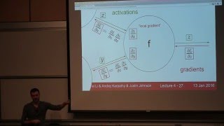
[Speaker:ANDREJ KARPATHY] OK, so let me dive into some administrative points first. So again, recall that assignment 1 is due next Wednesday. You have about 150 hours left. And I use hours because there's a more imminent sense of doom. And remember that a third of those hours you'll be unconscious. So you don't have that much time. It's really running out. And you might think that you have late days and so on, but these assignments just get harder over time, so you want to save those and so on. So start now. Let's see, so there's no office hours or anything like that on Monday. I'll hold makeup office hours on Wednesday because I want you guys to be able to talk to me about especially projects and so on. So I'll be moving my office hours from Monday to Wednesday. Usually I have my office hours at 6:00 PM. Instead, I'll have them at 5:00 PM, and usually it's in Gates 2 in Gates 259, so minus 1 on both. And yeah. And also to note, when you're going to be studying for midterm that's coming up in a few weeks, make sure you go through the lecture notes as well, which are really parts of this class. And I kind of pick and choose some of the things that I think are most valuable to present in a lecture, but there's quite a bit of more material to be aware of that might pop up in the midterm, even though I'm covering some of the most important stuff usually in the lecture. So do read through those lecture notes there. Complementary to the lectures. And so the material for the midterm will be drawn from both the lectures and the notes. OK. So having said all that, we're going to dive into the material. So where we are right now, just as a reminder, we have the score function. We've looked at several loss functions, such as the SVM loss function last time. And we looked at the full loss that you achieve for any particular set of weights. On— over your training data. And this loss is made up of two components. There's a data loss and a regularization loss, right? And really what we want to do is we want to derive now the gradient expression of the loss function with respect to the weights. And we want to do this so that we can actually perform the optimization process. And in the optimization process, we're doing a gradient descent where we iterate evaluating the gradient on your weights, doing a parameter update, and just repeating this over and over again. So that we're converging to the low points of that loss function. And when we arrive at a low loss, that's equivalent to making good predictions over our training data in terms of the scores that come out. Now, we also saw that there are two kind of ways to evaluate the gradient. There's a numerical gradient, and this is very easy to write, but it's extremely slow to evaluate. And there's an analytic gradient, which is— which you obtain by using calculus, and we'll be going into that in this lecture quite a bit more. And so it's fast, exact, which is great. But it's not— you can get it wrong sometimes. And so we always perform what we call gradient check, where we write all the expressions to compute the analytic gradient, and then we double-check its correctness with numerical gradient. And so I'm not sure if you're going to see that. You're going to see that definitely in the assignments. OK, so now you might be tempted to— when you see this setup, we just want to derive the gradient of the loss function with respect to the weights, you might be tempted to just, you know, write out the full loss and just start to take the gradients as you see in your calculus class. But the point I'd like to make is that you should think much more of this in terms of computational graphs instead of, instead of just taking— thinking of one giant expression that you're going to derive on pen— with pen and paper, the expression for the gradient. And the reason for that— so here we're thinking about these values flow— flowing through a computational graph where you have these operations along circles. And they trans— they're basically little function pieces that transform your inputs all the way to the loss function at the end. So we start off with our data and our parameters as inputs. They feed through this computational graph, which is just all these series of functions along the way, and at the end we get a single number, which is the loss. And the reason that I'd like you to think about it this way is that these expressions right now look very small, and you might be able to derive these gradients, but these expressions are— and computational graphs are about to get very big. And so for example, convolutional neural networks will have hundreds, maybe, or dozens of operations. So we'll have all these images flowing through, like, pretty big computational graph to get our loss. And so it becomes impractical to just write out these expressions. And convolutional networks are not even the worst of it. Once you actually start to, for example, do something called a neural Turing machine, which is a paper from DeepMind, where this is basically a differentiable Turing machine. So the whole thing is differentiable, the whole— procedure that the computer is performing on the tape is made smooth and is differentiable computer basically. And the computational graph of this is huge. And not only is this— this is not it because what you end up doing, and we'll go into recurrent neural networks in a bit, but what you end up doing is you end up unrolling this graph. So think about this graph copied many hundreds of time steps. And so you end up with this giant monster of hundreds of thousands of nodes and little computational units. And so it's impossible to write out, you know, here's the loss for the neural Turing machine. It's just impossible. It would take like billions of pages. And so we have to think about this more in terms of data structures of little functions transforming intermediate variables to get us the loss at the very end. Okay? So we're going to be looking specifically at computational graphs and how we can derive the gradient on the inputs with respect to the loss function at the very end. Okay? So let's start off simple and concrete. Uh, so let's consider a very small computational graph where we have 3 scalars as inputs to this graph, x, y, and z, and they take on these specific values in this example of -2, 5, and -4. And we have this very small, um, graph or circuit. You'll hear me refer to these interchangeably either as a graph or a circuit. So we have this graph that at the end gives us, um, this output -12, okay? So here what I've done is I've already prefilled what we'll call the forward pass of this graph. Where I set the inputs and then I compute the outputs, okay? And now what we'd like to do is we'd like to derive the gradients of the expression on the inputs. And so what we'll do now is I'll introduce this intermediate variable q after the plus gate. So there's a plus gate and a times gate, as I'll refer to them. And this plus gate is computing this output q. And so q is this intermediate as a result of x y, and then f is a multiplication of q and z. And what I've written out here is basically what we want is the gradients, the derivatives df/dx, df/dy, df/dz. And I've written out the intermediate, these little gradients for every one of these two expressions separately. So now we've performed the forward pass going from left to right. And what we'll do now is we'll derive the backward pass. We'll go from the back to the front computing gradients of all the intermediates in our circuit until at the very end we're going to be left with the gradients on the inputs. And so we start off at the very right. And as a base case of this recursive procedure, we're considering the gradient of f with respect to f. So this is just the identity function. So what is the derivative of just identity mapping? What is the gradient of df by df? It's 1, right? So the identity has a gradient of 1. So So that's our base case— we start off with 1. And now we're going to go backwards through this graph. So we want the gradient of f with respect to z. Um, so what is that in this computational graph?

x y q.

Okay, it's Q. So we have that written out right here. And what is Q in this particular example? It's, uh, 3, right? So the gradient on z according to this will become just 3. So I'm going to be writing the gradients under the lines in red, and the values are in green above the lines. So we have the gradient on the— in the front is 1, and now the gradient on z is 3. And what red 3 is telling you really intuitively— keep in mind the interpretation of a gradient— is what that's saying is that the influence of z on the final value is positive and with sort of a force of 3. So if I increment z by a small amount h, then the output of the circuit will react by increasing, because it's a positive 3, will increase by 3H. So a small change will result in a positive change on the output. Now the gradient on Q in this case will be— so df/dQ is z. What is z? -4. Okay. So we get a gradient of -4 on that path of the circuit. And what that's saying is that if Q were to increase, then the output of the circuit will decrease, okay? By— if you increase by h, the output of the circuit will decrease by 4h. That's the slope, is -4. Okay, now we're going to continue this recursive process through this plus gate, and this is where things get slightly interesting, I suppose. So we'd like to compute the gradient on f on y with respect to y. And so the gradient on y with this, um, in this particular graph will become What's the right answer? Let's just guess, and then we'll see how this gets derived properly. [Speaker:AUDIENCE] Negative 4. [Speaker:ANDREJ KARPATHY] So I hear some murmurs of the right answer. It will be negative 4. So let's see how— so there are many ways to derive it at this point, because the expression is very small, and you can kind of glance at it. But the way I'd like you to think about this is by applying chain rule, OK? So the chain rule says that if you would like to derive the gradient of f on y, then it's equal to df/dq times dq/dy, right? And so we've computed both of those expressions. In particular, dq/dy we know is -4. So that's the effect of— the influence of q on f is df/dq, which is -4. And now we know the loc— we'd like to know the local influence of y on q. And that local influence of y on q is 1, because that's the local— as I'll refer to as the local derivative of y for the plus gate. And so the chain rule tells us that the correct thing to do to chain these two gradients, the local gradient of y on Q and the kind of global gradient of Q on the output of the circuit, is to multiply them. So we'll get -4 times 1. And so this is kind of the, the crux of how backpropagation works. This is very important to understand here, that we have these two pieces that we keep multiplying through when we perform this chain rule. We have Q computed x y, and the derivative on x and y with respect to that single expression is 1 and 1. So keep in mind the interpretation of the gradient. What that's saying is that x and y have a positive influence on Q, uh, with a slope of 1. So increasing x by h will increase Q by h. Okay? And now what we eventually like is we'd like the influence of y on the final output of the circuit. And so the way this ends up working is you take the influence of y on q, and we know the influence of q on the final loss, which is what we are recursively computing here through this graph. And the correct thing to do is to multiply them. So we end up with a negative 4 times 1, okay, negative 4. And so the way this works out is basically what this is saying is that the influence of y on the final output of the circuit is negative 4. So increasing y should decrease the output of the circuit by negative 4 times. The little change that you've made. And the way that ends up working out is y has a positive influence on q. So increasing y slightly increases q, which slightly decreases the output of the circuit. So chain rule is kind of giving us this correspondence. Go ahead.

In practice, would you store it in sort of like a variable format or in a symbol format, or would you store it in terms of what the other variables are?

Yeah, thank you. So we're going to get into this. You'll see many— basically, this entire class is about this. So you'll see many, many instantiations of this, and I'll drill this into you by the end of this class, and you'll understand it. You will not have any symbolic expressions anywhere once we compute this, once we're actually implementing this. And you'll see implementations of it later in this. It will always be just vectors and numbers, raw vectors, numbers. OK, and looking at x, we have a very similar thing that happens. We want df/dx. That's our final objective. But— and we have to combine it. We know what the x's— What is x's influence on q, and what is q's influence on the end of the circuit? And so that ends up being a chain rule. So you take -4 times 1, and it gives you -1. Okay? So the way this works, to generalize a bit from this example, and the way to think about it is as follows. You are a gate embedded in a circuit, and this is a very large computational graph or circuit. And you receive some inputs, some particular numbers, x and y, come in, and you perform some operation f on them and compute some output z. OK? And now, now this value of z goes into computational graph and something happens to it. But you're just a gate hanging out in a circuit and you're not sure what happens. But by the end of the circuit, the loss gets computed. OK? And that's the forward pass. And then we're proceeding recursively in the reverse order backwards. But before that, actually, before I get to that part, you've re— right away when I get x and y, the thing I'd like to point out that during the forward pass, if you're this gate and you get your values x and y, you compute your output z. And there's another thing you can compute right away, and that is the local gradients on x and y. So I can compute those right away because I'm just a gate and I know what I'm performing, like say addition or multiplication. So I know the influence that x and y have on my output value. So I can compute those guys right away. Okay? What— but then what happens near the end, so the loss gets computed and now we're going backwards. I'll eventually learn about what is my influence on the final output of the circuit, the loss. So I'll learn what is dL/dz in there. The gradient will flow into me. And what I have to do is I have to chain that gradient through this recursive case. So I have to make sure to chain the gradient through my operation that I performed. And it turns out that the correct thing to do here by chain rule, really what it's saying, is the correct thing to do is to multiply your local gradient with that gradient. And that actually gives you the dl/dx. That gives you the influence of x on the final output of the circuit. So really, chain rule is just this added multiplication where we take our— what I'll call global gradient of this gate on the output, and we chain it through the local gradient. And the same thing goes for y. So it's just a multiplication of that guy, that gradient, by your local gradient if you're a gate. And then remember that these x's and y's, they are coming from different gates, right? So you end up recursing this process through the entire computational circuit. And so these gates just basically communicate to each other the influence on the final loss. So they tell each other, OK, if this is a positive gradient, that means you're positively influencing the loss. And if it's a negative gradient, you're negatively influencing the loss. And these just get all multiplied through the circuit by these local gradients. And you end up with— and this process is called backpropagation. It's a way of computing through a recursive application of chain rule through computational graph the influence of every single intermediate value in that graph on the final loss function. And so we'll see many examples of this throughout this lecture. I'll go into a specific example that is slightly larger, and we'll work through it in detail. But I don't know if there are any questions at this point that anyone would like to ask. Go ahead. What happens if z is used by two other nodes? If z is used by multiple nodes, I'm going to come back to that. You add the gradients. The gradient, the correct thing to do is to add them. So if z is being influenced in multiple places in the circuit, the backward flows will add. But we'll come back to that point. Go ahead. What happens if you have a bunch of inputs to f, 100, 1,000, and the way you randomly initialize your weights, you end up that because your squashing function, the value of f is somewhere on the asymptote. So then when you're computing the gradient, the change in any one of the components will not really change the function output that much. Aren't you going to get trapped? So I think I would have repeated your question, but you're jumping ahead like 100 slides. So we're going to get to all of those issues. And we're going to see, yeah, you're going to get what we call vanishing gradient problems and so on. We'll see. Okay? Let's go through another example to make this more concrete. So here we have another circuit. It happens to be computing a little 2-dimensional sigmoid neuron, but for now don't worry about that interpretation. Just think of this as that's an expression. So 1 over 1 plus e to the whatever. So the number of inputs here is 5, and we're computing that function, and we have a single output over there. Okay? And I translated that mathematical expression into this computational graph form. So we have to recursively from inside out compute this expression. So we first do all the little, uh, w times x's, and then we add them all up, and then we, uh, take a negative of it, and then we exponentiate that, and then we add 1, and then we finally divide, and we get the result of the expression. And so what we're going to do now is we're going to backpropagate through this expression. We're going to compute what the influence of every single input value is on the output of this expression. What is the gradient here? Yeah, go ahead.

Is it a custom to use functions like plus or times as binary functions instead of multiple parity functions?

So for now, so you're concerned about the interpretation of plus maybe in these circles. For now, let's just assume that this plus is just a binary plus, is a binary plus gate. And we have there a plus 1 gate. I'm making up these gates kind of on the spot. And we'll see that what is a gate or is not a gate is kind of up to you. I'll come back to this point a bit— in a bit. So for now, I just like— we have several more gates that we're using throughout. And so I just like to write out as we go through this example several of these derivatives. So we have exponentiation. And we know for every little local gate what these local gradients are. So we can derive that using calculus. So e to the x derivative is e to the x, and so on. So these are all the operations, and also addition and multiplication, which I'm assuming that you have memorized in terms of what the gradients look like. So we're going to start off at the end of the circuit. And I've already filled in a 1.00 in the back, because that's how we always start this recursion, with a 1.0, right? Since that's the gradient on the identity function. Now we're going to backpropagate through this 1 over x operation, OK? The derivative of 1 over x, the local gradient, is negative 1 over x squared. So that 1 over x gate during the forward pass received input 1.37, and right away that 1 over x gate could have computed what the local gradient was. The local gradient was negative 1 over x squared. And now during backpropagation, it has to, by chain rule, multiply that local gradient by the gradient of it on the final output of the circuit, which is easy because it happens to be at the end. So what ends up being the expression for the backpropagated gradient here from the 1 over x gate? The chain rule always has two pieces, local gradient times the gradient from the top or from above. [Speaker:AUDIENCE] This is minus 1 over 1 plus e to the x squared. Minus— yeah, OK. Yeah, so that's correct. So we get -1 over x squared, which is the gradient df by dx. So that is the local gradient, -1 over 3.7 squared, and then multiplied by 1.0, which is the gradient from above, which is really just 1 because we've just started. And so I'm applying chain rule right away here, and the output is -0.53. So that's the gradient on that piece of the wire where this valley was flowing, OK? So it has a negative effect on the output. Um, and you might expect that, right? Because if you were to increase this value and then it goes through a gate of 1 over x, then if you increase this, then 1 over x gets smaller. So that's why you're seeing negative gradient, right? So we're going to continue backpropagation here. The next, uh, gate in the circuit, it's adding a constant of 1. So the local gradient, if you look at, uh, adding a constant to a value, the gradient of— on x is just 1. 1, right, by basic calculus. And so the chained gradient here that we continue along the wire will be— we have local gradient, which is 1, times the gradient from above the gate, which it has just learned is -0.53. OK? So -0.53 continues along the wire unchanged. And intuitively that makes sense, right? Because this, this value floats and it has some influence on the final circuit. And now if you're sk— if you're adding 1, then its influence, its rate of change, its slope towards the final value doesn't change. If you increase this by some amount, the effect at the end will be the same because the rate of change doesn't change through the +1 gate. It's just a constant offset. Okay, we continue derivation here. So the gradient of e^x is e to the x. So to continue backpropagation, we're going to perform— so this gate saw input of negative 1. It right away could have computed its local gradient. And now it knows that the gradient from above is negative 0.53. So to continue backpropagation here and applying chain rule, we would receive— [Speaker:AUDIENCE] Do you know why exactly? [Speaker:ANDREJ KARPATHY] OK. So these are mostly rhetorical questions. I'm not sure. But yeah, basically e to the negative 1, which is e to the x, the x input to this x gate, times the chain rule, right? So the gradient from above is negative 0.53, so we keep multiplying that on. So what is the effect on me, and what do I have an effect on the final end of the circuit? Those are being always multiplied. So we get negative 0.2 at this point. So now we have a times negative 1 gate. So what ends up hap— what happens to the gradient when you do a times negative 1 in the computational graph? [Speaker:AUDIENCE] Negative 1. It flips around, right? Because we have basically a constant multiply of input, which happened to be a constant of -1. So -1 times— 1 times -1 gave us -1 in the forward pass. And so now we have to multiply by a, that's the local gradient, times the gradient from above, which is 0.2. So we end up with just positive 0.2 now. So we're now continuing backpropagation. We're backpropagating plus. And this plus operation has multiple inputs here. The gradient, the local gradient for the plus gate is 1 and 1. So what ends up happening to— what gradients flow along the output wires? So the plus gate has a local gradient on all of its inputs always will be just 1, right? Because if you just have a function, you know, x y, then for that function, the gradient on either x or y is just 1. And so what you end up getting is just 1 times 0.2. And so in fact, for a plus gate, always you see the same fact where the local gradient on all of its inputs is 1. And so whatever gradient it gets from above, it just always distributes gradient equally to all of its inputs because in the chain rule, they'll get multiplied. And when you multiply by 1, something remains unchanged. So a plus gate is kind of like a gradient distributor, where if something flows in from the top, it will just spread out all the gradients equally to all of its children. And so we've already received one of the inputs is gradient 0.2 here on the very final output of the circuit. And so this influence has been computed through a series of applications of chain rule along the way. So now let's— there was another plus gate that I've skipped over. And so this 0.2 kind of distributes to both 0.2, 0.2 equally. So we've already done a plus gate. And there's a multiply gate there. And so now we're going to backpropagate through that multiply operation. And so the local grade— so what will be the gradients for w0 and x0? What will be the gradient for w0 specifically? Someone say 0? 0 would be wrong. It will be— so the gradient w1 will be— w0, sorry, will be -1 times 0.2. Good. And the gradient on x0 will be— there's a bug, by the way, in the slide that I just noticed like a few minutes before I actually created the class. So it created the— started the class. So you see 0.39 there? It should be 0.4. It's because of a bug in the visualization because I'm truncating at 2 decimal digits. Anyways, but basically that should be 0.4 because the way you get that is 2 times 0.2 gives you 0.4, just like I've written out over there. So that's what the output should be there. Um, okay, so that— so we've backpropagated this circuit here, uh, and we've backpropagated through this expression. And so you might imagine in our actual downstream applications, We'll have data and all the parameters as inputs. The loss function is at the top at the end. So we'll do forward pass to evaluate the loss function. And then we'll backpropagate through every piece of computation we've done along the way. And we'll backpropagate through every gate to get our inputs. And backpropagate just means apply chain rule many, many times. And we'll see how that is implemented in a bit. Sorry, did you have a question?

I don't know, just w1 and x1.

Oh, yeah, so I'm going to skip that because it's the same. So I'm going to skip the other type timescale. Any other questions at this point?

So this process takes on the order of the same time it takes to forward propagate?

That's right. So the cost of forward and backward propagation is roughly equal.

Is it actually within a constant? Do you know what the constant is?

Well, it should be. It almost always ends up being basically equal when you look at timings. Usually the backward pass is slightly slower. But yeah. OK. So let's see. One thing I wanted to point out before we move on is that the setting of these gates— like, these gates are arbitrary. So one thing I could have done, for example, is— some of you may know this— I can collapse these gates into one gate if I wanted to. For example, there's something called the sigmoid function, which has that particular form. So sigma of x, which is the sigmoid function, computes 1 over 1 plus e to the minus x. And so I could have rewritten that expression and I could have collapsed all of those gates that made up the sigmoid gate into a single sigmoid gate. And so there's a sigmoid gate here, and I could have done that in a single go, sort of. And what I would have had to do if I wanted to have that gate is I need to compute an expression for how this, um, so what is the local gradient for the sigmoid gate basically? So what is the gradient on the sigmoid gate on its input? And I have to go through some math, which I'm not going to go into detail, but you end up with that expression over there. It ends up being 1 minus sigmoid of x times sigmoid of x. That's the local gradient. And that allows me to now put this piece into a computational graph, because once I know how to compute the local gradient, everything else is defined just through chain rule and multiplying everything together. So we can backpropagate through this sigmoid gate now. And the way that would look like is the input to the sigmoid gate was 1.0. That's what flew— went into the sigmoid gate and 0.73 went out. So 0.73 is sigma of x. Okay? And now we want the local gradient, which is, as we've seen from the math that I performed there, 1 minus sigma of x times sigma of x. So you get sigma of x is 0.73, multiplying 1 minus 0.73, that's the local gradient. And then times— well, we happen to be at the end of the circuit, so times 1.0, which I'm not even writing. So we end up with 0.2. And of course, we get the same answer, 0.2, as we received before, 0.2, because calculus works. But basically, we could have broken up this expression down and did one piece at a time, or we could just have a single sigmoid gate. And that's kind of up to us at what level of hierarchy do we break these expressions. And so you'd like to intuitively cluster these expressions into single gates if it's very efficient or easy to derive the local gradients, because then those become your pieces.

[Speaker:AUDIENCE] Do libraries— Do libraries typically do that where they notice, oh, they say that's a sigmoid, I know how to do that fast?

Yes. So the question is, do libraries typically do that? Do they worry about what's easy to or convenient to compute? And the answer is, yeah, I would say so. So if you notice that there's some piece of operation you'd like to do over and over again, and it has a very simple local gradient, then that's something very appealing to actually create a single unit out of. And we'll see some of those examples actually in a bit, I think. Okay, I'd like to also point out that once you— the reason I like to think about these computational graphs is it really helps your intuition to think about how gradients flow in a neural network. It's not just, you don't want this to be a black box to you, you want to understand intuitively how this happens. And you start to develop after a while of looking at computational graphs intuitions about how these gradients flow. And this, by the way, helps you debug some issues like, say, we'll go to vanishing gradient problem. It's much easier to understand exactly what's going wrong in your optimization if you understand how gradients flow in networks. It will help you debug these networks much more efficiently. And so some intuitions, for example, we already saw that the 8th add gate, it has a local gradient of 1 to all of its inputs. So it's just a gradient distributor. That's like a nice way to think about it. Whenever you have a plus operation anywhere in your score function or your ConvNet or anywhere else, it just distributes gradients equally. The MAX gate is instead a gradient router. And the way this works is if you look at the expression like we have— oh, great, these markers don't work. So if we have a very simple binary expression of max of xy, so if this is a gate, then the gradient on x and y, if you think about it, the gradient on the larger one of your inputs, whichever one was larger, the gradient on that guy is 1. And all this— and the smaller one has a gradient of 0. And intuitively, that's because if one of these was smaller, then wiggling it has no effect on the output because the other guy is larger, and that's what ends up propagating through the gate. So you end up with a gradient of 1 on the larger one of the inputs. And so that's why MaxGate is a gradient router. If I'm a MaxGate and I have received several inputs, one of them was largest of all of them, and that's the value that I propagated through the circuit, at backpropagation time, I'm just going to receive my gradient from above, And I'm going to route it to whoever was my largest input. So it's a gradient router. And the multiply gate is a gradient switcher. I actually don't think that's a very good way to look at it. But I'm referring to the fact that it's not actually— never mind about that part. Go ahead. What happens if for one of your max gates, its two inputs are equal? What happens to the backward propagation? So yeah, so your question is what happens if the two inputs are equal when you go through max gate? Yeah, what happens? [Speaker:AUDIENCE] Probably just pick one of them arbitrarily, whichever one you encounter. [Speaker:ANDREJ KARPATHY] Yeah, you pick one. Yeah, I don't think it's correct to distribute it to all of them. I think you'd have to pick one. Yeah, but that basically never happens in actual practice. Max gradient here, actually I have an example. So z here was larger than w. So only z has an influence on the output of this max gate, right? So when 2 flows into the max gate, it gets routed to z. And w gets a 0 gradient because its effect on the circuit is nothing. There's 0. Because when you change it, it doesn't matter when you change it because z is the larger value going through the computational graph. I have another note that is related to backpropagation, which we already addressed through a question. I just wanted to briefly point out with a terribly bad-looking figure that if you have these circuits, and sometimes you have a value that branches out into a circuit and is used in multiple parts of the circuit, the correct thing to do by multivariate chain rule is to actually add up the contributions at the operation. So gradients add when they backpropagate backwards through the circuit. If they ever flow, they add up in this backward flow. All right, we're going to go into implementation very soon. I'll just take some more questions. Is there a closed loop case instead of open loop? Thank you for the question. The question is, is there ever, like, loop in these graphs? There will never be loops. So there are never any loops. You might think that if you use a recurrent neural network that there are loops in there, but there's actually no loops. Because what we'll do is we will take a recurrent neural network and we'll unfold it through time steps. And this will all become— there will never be a loop in the unfolded graph where we've copy-pasted that small return that piece over time. You'll see that more when we actually get into it. But these are always DAGs. There's no loops. OK, awesome. So let's look at implementation and how this is actually implemented in practice. And I think it will help make this more concrete as well. So we always have these graphs, computational graphs. These are the best way to think about structuring neural networks. And so what we end up with is all these gates that we're going to see in a bit. But on top of the gates, there's something that needs to maintain connectivity structure of this entire graph, what gates are connected to each other. And so usually that's handled by a graph or a net object, usually a net. And the net object has these two main pieces, which is the forward and the backward piece. And this is just pseudocode, so this won't run. But basically, roughly the idea is that in the forward pass, we're iterating over all the gates in the circuit that— and they're sorted in topological order. What that means is that all the inputs must come to every node before the output can be consumed. So these are just ordered from left to right, and we're just forwarding— we're calling a forward on every single gate along the way. So we iterate over that graph, and we just go forward on every single piece, and this net object will just make sure that that happens in the proper connectivity pattern. And in the backward pass, we're going in the exact reversed order, and we're calling backward on every single gate, and these gates will end up communicating gradients to each other, and they all get chained up. And computing the analytic gradient at the back. So really, a net object is a very thin wrapper around all these gates, or as we'll see, they're called layers. Layers or gates, I'm going to use those interchangeably. And they're just very thin wrappers around connectivity structure of these gates and calling a forward and backward function on them. And then let's look at a specific example of one of the gates and how this might be implemented. And this is not just the pseudocode. This is actually more, like, correct implementation in some sense. Like, this might run at the end. So let's consider a multiply gate and how it could be implemented. A multiply gate in this case is just a binary multiply, so it receives two inputs, x and y. It computes their multiplication, z is x times y, and it returns z. And all these gates must basically satisfy this API of a forward call and a backward call. How do you behave in a forward pass and how do you behave in a backward pass? And in a forward pass, we just compute whatever. In a backward pass, we eventually end up learning about what is our gradient on the final loss. So dl/dz is what we learn. That's represented in this variable dz. And right now everything here is scalars. So x, y, z are numbers here. dz is also a number telling the influence on the end of the circuit. And what this gate is in charge of in this backward pass is performing the little piece of chain rule. So what we have to compute is how do you chain this gradient dz into your inputs x and y. In other words, we have to compute dx and dy, and we have to return those in the backward pass. And then the computational graph will make sure that these get routed properly to all the other gates. And if there are any edges that add up, the computational graph might add all those gradients together. OK, so how would we implement the dx and dy? So for example, what is dx in this case? What would it be equal to, the implementation? Y times dz. Great. And so y times dz. Additional point to make here, by the way, note that I've added some lines in the forward pass. We have to remember these values x and y because we end up using them in the backward pass. So I'm assigning them to a self dot because I need to remember what x, y are because I need access to them in my backward pass. In general, in backpropagation, when we build these when you actually do the forward pass, every single gate must remember the inputs and any kind of intermediate calculations that it has performed that it needs to do— that needs access to in the backward pass. So basically, when we end up running these networks at runtime, just always keep in mind that as you're doing this forward pass, a huge amount of stuff gets cached in your memory, and that all has to stick around because during backpropagation you might need access to some of those variables. And so your memory ends up ballooning up during the forward pass, and then in backward pass it gets all consumed, and we need all those intermediates to actually compute the proper backward pass. So that's—

[Speaker:AUDIENCE] You can do a forward pass if you're not going to do a backward pass fast, like a lot faster.

[Speaker:ANDREJ KARPATHY] Yeah, so if you know you don't want to do backward pass, then you can get rid of many of these things, and you don't need to cache them. So you can save on memory for sure. But I don't think most implementations actually worry about that. I don't think there's a lot of logic that deals with that. Usually we end up remembering it anyway.

Well, it does seem like if you want to test on your validation set, that's way faster than just doing one pass through your training.

I see. Yeah, so I think if you're in an embedded device, for example, and you worry really about your memory constraints, this is something that you might take advantage of. If you know that a neural network only has to run at test time, then you might want to make sure to go into the code and make sure nothing gets cached in case you want to do a backward pass. Questions? Yes? If you are computing your local gradients during the forward pass, [INAUDIBLE] You're saying if we remember the local gradients in the forward pass, then we don't have to remember the other intermediates? I think that might only be the case in some simple expressions like this one. I'm not actually sure if that's true in general. But I mean, you're in charge of— remember whatever you need to perform the backward pass. On a gate-by-gate basis. You don't— you can remember whatever you feel like has lower footprint and so on. And you can be clever with that. OK, so just to give you guys an example of what this looks like in practice, we're going to look at specific examples, say, in Torch. Torch is a deep learning framework, which we might go into a bit near the end of the class, that some of you might end up using for your projects. If you go into the GitHub repo for Torch and you look at— Basically, it's just a giant collection of these layer objects, and these are the gates. Layers, gates, the same thing. So there's all these layers. That's really what a deep learning framework is, is just a whole bunch of layers and a very thin computational graph thing that keeps track of all the layer connectivity. And so really, the image to have in mind is all these things are your Lego blocks, and then we're building up these computational graphs out of your Lego blocks, out of the layers. You're putting them together in various ways depending on what you want to achieve. And so you end up building all kinds of stuff. So that's how you work with neural networks. So every library is just a whole set of layers that you might want to compute. And every layer is just implementing a small function piece. And that function piece knows how to do a forward, and it knows how to do a backward. So just with this specific example, let's look at the mul_constant layer in Torch. The mul_constant layer performs just a scaling by a— scalar. So it takes some tensor x. So this is not just a scalar, but it's actually like an array of numbers basically. Because when we actually work with these, we do a lot of vectorized operations. So we receive a tensor, which is really just an n-dimensional array, and we scale it by a constant. And you can see that this layer actually just has 40 lines. There's some initialization stuff. This is Lua, by the way, if this is looking some foreign to you. But there's initialization where you actually pass in that A that you want to use as your scaling. And then during the forward pass, which they call update_output, in a forward pass, all they do is they just multiply Ax and return it. And in the backward pass, which they call update_grad_input, uh, there's an if statement here, but really when you look at these three lines that are most important, you can see that all it's doing is it's copying into a variable grad_input, which it needs to compute. That's your gradient that you're passing up. The grad_input is, you're copying grad_output. grad_output is your gradient on the final loss. You're copying that over into grad_input, and you're multiplying by the scalar, which is what you should be doing because your local gradient is just a. And so you take the output you have, you take the gradient from above, and you just scale it by a, which is what these three lines are doing. And that's your grad_input, and that's what you return. So that's one of the hundreds of layers that are in Torch. We can also look at examples in Caffe. Caffe is also a deep learning framework specifically for images that you might be working with. Again, if you go into the layers directory in GitHub, you just see all these layers. All of them implement the forward-backward API. So just to give you an example, there's a sigmoid layer in Caffe. So sigmoid layer takes a blob. So Caffe likes to call these tensors blobs. So it takes a blob— it's just an n-dimensional array of numbers— and it passes it element-wise through a sigmoid function. And so it's computing in the forward pass a sigmoid. Which you can see there. Let me use my pointer. Okay. So there it's calling— so a lot of this stuff is just boilerplate, getting pointers to all the data. And then we have a bottom blob, and we're calling a sigmoid function on the bottom, and that's just the sigmoid function right there. So that's what we compute. And in the backward pass, uh, some boilerplate stuff, but really what's important is we need to compute the gradient times the chain rule here. So that's what you see in this line. That's where the magic happens. Where we take the diff. So they call the gradients diffs. And you compute the bottom diff as the top diff times this piece, which is really the— that's the local gradient. So this is chain rule happening right here through that multiplication. And that's it. And so every single layer, just the forward-backward API. And then you have a computational graph on top, or a net object that keeps track of all the connectivity. Any questions about some of these implementations and so on? Go ahead. [Speaker:AUDIENCE] So do we have to go through the entire forward and backward step for every update step? [Speaker:ANDREJ KARPATHY] Yes, thank you. So the question is, do you have to go through forward and backward for every update? The answer is yes, because when you want to do update, you need the gradient. And so you need to do forward on your— you sample a mini batch, you do a forward, you right away do a backward, and now you have your analytic gradient. And now I can do an update. Where I take my analytic gradient and I change my weights a tiny bit in the direction, the negative direction of your gradient. So forward computes the loss, backward computes your gradient, and then the update uses the gradient to increment your weights a bit. So that's what keeps happening in the loop. When you train a neural network, that's all that's happening. Forward, backward, update, forward, backward, update. We'll see that in a bit. Go ahead. [Speaker:AUDIENCE] The reason for having for loop there is simply because this is for [Speaker:ANDREJ KARPATHY] You're asking about the for loop? Oh, is there a for loop here? I didn't even notice. OK. Yeah, they have a for loop. Yeah, so you'd like this to be vectorized. I'm not actually sure. Oh, because this is C++. So I think, yeah, they just do it. Go for it.

Yeah, yeah.

So this is a CPU implementation, by the way. I should mention. That this is a CPU implementation of the sigmoid layer. There's a second file that implements the sigmoid layer on GPU, and that's CUDA code. And so that's a separate file. It would be sigmoid.cu or something like that. I'm not showing you that. Any other questions? OK, great. So one point I'd like to make is we'll be, of course, working with vectors. So these things flowing along our graphs are not just scalars. They're going to be entire vectors. And so nothing changes. The only thing that is different now, since these are vectors— x, y, and z are vectors— is that this local gradient, which before used to be just a scalar, now they're in general, for general expressions, they're full Jacobian matrices. And so Jacobian matrix is this two-dimensional matrix, and basically tells you what is the influence of every single element in x on every single element of z. And that's what Jacobian matrix stores. And the gradient is the same expression as before, but now, say here dz by dx is a vector and dl by dz, um, is, um, sorry, dl by dz is a vector and dz by dx is an entire Jacobian matrix. So you end up with an entire matrix vector multiply to actually chain the gradient backwards.

If you only have one output, do you still have, uh, two-dimensional gradient as you go backward?

Um, no. So I'll come back to this point in a bit. You never actually end up forming the full Jacobian. You'll never actually do this matrix multiply most of the time. This is just a general way of looking at, you know, arbitrary function, and I need to keep track of this. And I think that these two are actually out of order, because dz/dx is the Jacobian, which should be on the left side. So that's a— I think that's a mistake in the slide, because this should be a matrix-vector multiply. So I'll show you why you don't actually need to ever form those Jacobians. So let's work with a specific example that is relatively, uh, common in neural networks. Suppose we have this nonlinearity max of 0 and x. So really what this is— operation is doing is it's receiving a vector, say, of 4,096 numbers, which is a typical thing you might want to do. 4,096 numbers, real-valued, come in, and you're computing an element-wise thresholding at 0. So anything that is lower than 0 gets clamped to 0, and that's your function that you're computing. And so output vector is of the same dimension. Um, so the question here I'd like to ask is, what is the size of the Jacobian matrix for this layer? 4,096 by 4,096. In principle, every single number in here could have influenced every single number in there. But that's not the case necessarily, right? So the second question is, So this is a huge matrix, 16 million numbers. But why would you never form it? What does the Jacobian actually look like?

Wouldn't it— because it's element-wise, wouldn't it just be a vector?

No, Jacobian will always be a matrix, because every one of these 4,096 could have influenced every—

I thought you said it's element-wise.

It is. So the Jacobian is still a giant 4,096 by 4,096 matrix, but it has special structure, right? And what is that special structure? Good.

[Speaker:AUDIENCE] It's diagonal even when some are even zeros.

[Speaker:ANDREJ KARPATHY] Yeah. So this Jacobian is huge. So it's 4,096 by 4,096 matrix. But there's only elements on the diagonal because this is an element-wise operation. And moreover, they're not just ones. But for whichever element was less than 0, it was clamped to 0. So some of these ones actually are zeros in whichever elements had a lower than 0 value during the forward pass. And so the Jacobian would just be almost an identity matrix, but some of them are actually 0. So you never actually would want to form the full Jacobian because that's silly. And so you'd never actually want to carry out this operation as a matrix-vector multiply because there's special structure that we want to take advantage of. And so in particular, the gradient— the backward pass for this operation is very, very easy because you just want to look at all the dimensions where your input was less than 0. And you want to kill the gradient in those dimensions. You want to set the gradient to 0 in those dimensions. So you take the grad output here, and whichever numbers were less than 0, just set them to 0. Set those gradients to 0, and then you continue backward pass. So very simple operations in the end in terms of efficiency.

In the backward pass, you always just report back a vector for each of the inputs.

That's right.

You never actually— [Speaker:AUDIENCE] You could do a matrix if you needed to in your internal state. But when you actually report back, you're always just a vector.

[Speaker:ANDREJ KARPATHY] Yeah, so the question is the communication between the gates is always just vectors. That's right. So this Jacobian, if you wanted to, you can form that. But that's internal to you inside the gate. And you can use that to do backprop. But what's going back to other gates, they only care about the gradient vector.

Unless you wind up having multiple outputs overall in your entire network.

Yes. So the question is, unless you end up having multiple outputs, because then for each output we have to do this. And so you'd— yeah. So we'll never actually run into that case because we almost always have a single output scalar value at the end because we're interested in loss functions. So we just have a single number at the end that we're interested in computing gradients with respect to. If we had multiple outputs, then we have to keep track of all of those as well. In parallel when we do the backpropagation. But we just have scalar-valued loss functions, so we don't have to worry about that. OK, make sense? So I wanted to also make the point that actually 4,096 dimension is not even crazy. Usually we use mini-batches. So say a mini-batch of 100 elements going through at the same time. And then you'd end up with 100 4,096-dimensional vectors that are all coming in in parallel. But all the examples in a mini-batch are processed independently of each other in parallel. And so this Jacobian matrix really ends up being 400 million— 400,000 by 400,000, so huge. So you never form these, basically. And you take care to actually take advantage of the sparsity structure in that Jacobian. And you hand-code operations. You don't actually write the fully generalized chain rule inside any gate implementation. OK, cool. So I'd like to point out that in your assignment, you'll be writing SVMs and softmax and so on. And I just kind of wanted to give you a hint on the design of how you actually should approach this problem. What you should do is just think about it as backpropagation, even if you're doing this linear classification optimization. So roughly, your structure should look— it looks something like this, where, again, stage your computation in units. That you know the local gradient of, and then do backprop when you actually evaluate these gradients in your assignment. So in the top, your code will look something like this, where we don't have any graph structure because you're doing everything inline. So no crazy edges or anything like that that you have to do. You will do that in the second assignment. You'll actually come up with a graph object, and you'll implement your layers. But in the first assignment, you're just doing it inline, just a straight-up vanilla setup. And so compute your scores based on w and x. Compute these margins which are max of 0 and the score differences, um, compute the loss, and then do backprop. And in particular, I would really advise you to have this intermediate scores that you create. It's a matrix, and then compute the gradient on scores before you compute the gradient on your weights. And so chain— use chain rule here. Otherwise, you're— like, you might be tempted to try to just derive w— the gradient on w equals, and then implement that, and that's an unhealthy way of approaching the problem. So stage your computation and do backprop through this course, and they will help you out. Um, okay, cool. So, let's see, some— the summary so far, neural networks are hopelessly large, so we end up with these computational structures and these intermediate nodes. Forward-backward API for both the neural network and the neural network is really a very thin wrapper around all these layers, and it handles all the communication between them. And this communication is always along like vectors being passed around. In practice, when we write these implementations, what we're passing around are these n-dimensional tensors. Really what that means is just an n-dimensional array, so like a NumPy array. Those are what goes between the gates. And then internally, every single gate knows what to do in the forward and backward pass. OK, so at this point, I'm going to end with backpropagation. And I'm going to go into neural networks. So any questions before we move on from backprop? Go ahead.

Yeah, in the last slide, the summation symbol, is that sort of handled with the fact that we're using matrices instead of vectors? Or how is the summation symbol?

The summation inside li equals blah? Yeah. Yeah, so there's a sum there. So you'd want that to be a vectorized operation that you— yeah, so basically the challenge in your assignment almost is how do you make sure that you do all of this efficiently, nicely with matrix vector operations in NumPy? So that's going to be some of the brain teaser stuff that you guys are going to have to do.

[Speaker:AUDIENCE] So you wouldn't implement a gate for that? You would make that implicit in the structure of the variable?

[Speaker:ANDREJ KARPATHY] Yeah, so it's up to you what you want your gates to be like and what you want them to be. [Speaker:AUDIENCE] But that wouldn't be one big plus gate, right? [Speaker:ANDREJ KARPATHY] Yeah, I don't think you'd want to do that. Yeah, I'm not sure. Maybe that works. I don't know. But yeah, it's up to you to design this and to backprop through it. Yeah, so that's fun. OK, so we're going to go to neural networks. This is exactly what they look like. So you'll be implementing these. And this is just what happens when you search on Google Images for neural networks. This is, I think, the first result or something like that. So let's look at neural networks. And before we dive into neural networks, actually, I'd like to do it first without all the brain stuff. So forget that they're neural. Forget that they have any relation whatsoever to a brain. They don't, but forget if you thought that they did, that they do. Let's just look at score functions, where before we saw that f wx is what we've been working with so far. But now, as I said, we're going to start to make that f more complex. And so if you wanted to use a neural network, then you're going to change that equation to this. So this is a two-layer neural network, and that's what it looks like. And it's just a more complex mathematical expression of x. And so what's happening here is you receive your input x and you multiply it by matrix just like we did before. Now what's come next— what comes next is a non-linearity or activation function, and we're going to go into several choices that you might make for these. In this case, I'm using the thresholding at 0 as an activation function. So basically we're doing matrix multiply, we threshold everything negative to 0, and then we do one more matrix multiply, and that gives us our scores. And so if I was to draw this, say, in case of CIFAR-10, we have 3,072 numbers going in. Those are the pixel values. And before, we just went one single matrix multiply to scores. We went right away to 10 numbers. But now we get to go through this intermediate representation of a hidden, a hidden state. We'll call them hidden layers. So hidden vector h of 100 numbers, say, or whatever you want your size of your neural network to be. So this is a hyperparameter that say that 100, and we go through this intermediate representation. So matrix multiply gives us 100 numbers, threshold at 0, and then one more matrix multiply to get the scores. And since we have more numbers, we have more wiggle to do more interesting things. So a more— one particular example of something interesting you might want to— what you might think that a neural network could do is going back to this example of interpreting linear classifiers on CIFAR-10. And we saw that the car class has this red car that tries to merge all the modes of different cars facing different directions. And so in this case, one single layer— one single linear classifier had to go across all those modes, and we couldn't deal with, for example, cars of different colors. That wasn't very natural to do. But now we have 100 numbers in this intermediate, and so you might imagine, for example, that one of those numbers could be just picking up on red car facing forward. Is just classifying, is there a red car facing forward? Another one could be red car facing slightly to the left, left car facing slightly to the right. And those elements of H would only become positive if they find that thing in the image. Otherwise, they stay at 0. And so another H might look for green cars or yellow cars or whatever else in different orientations. So now we can have a template for all these different modes. And so these neurons turn on or off if they find —and then this W2 matrix can sum across all those little car templates. So now we have, like, say, 20 car templates of what cars could look like. And now to compute the score of car classifier, there's an additional matrix multiply. So we have a choice of doing a weighted sum over them. And so if any one of them turn on, then through my weighted sum with positive weights, presumably, I would be adding up and getting a higher score. And so now I can have this multimodal car classifier through this additional hidden layer in between there. So that's a hand-wavy reason for why these would do something more interesting. Was there a question? Yeah. So let's say the H layer has less than 10 units. Would it then be always inferior than just using a linear classifier? So the question is, if H had— "less than 10 units, would it be inferior to a linear classifier?" I think that's actually not obvious to me. It's an interesting question. I think you could make that work. I think you could make it work. Yeah, I think that would actually work. Someone should try that for extra points on the assignment. So you'll have a section on the assignment, do something fun or extra. And so you get to come up with whatever you think is an interesting experiment, and we'll give you some bonus points. So that's a good candidate for something you might want to investigate, whether that works or not. Any other questions? Good.

So are there 100 of those car-facing left, car-facing right source of features per class, per each of the 10 classes, or is it for all of the 10 classes?

Sorry, I don't think I understood the question.

So you said there might be certain elements in the H vector that represent certain things —like the car facing left or facing right. Yep. Um, do each of the 10 classes have 100 different—

I see. Uh, so you're really asking about the layout of the H vector and how it gets allocated over the different modes of the dataset. And I don't have a good answer for that. This— since we're going to train this fully with backpropagation, uh, I, I think it's slightly naive to think that there will be exact template for, say, a left car facing— red car facing left. You probably won't find that. You'll find these kind of like mixes. And weird things, intermediates, and so on. So this neural network will come in and it will optimally find a way to truncate your data with its linear boundaries, and these weights will all get adjusted just to come— make it come out right. So it's really hard to say, it will become tangled up, I think. Good. I understand, but so, uh, the number 100 for h was like chosen arbitrarily? That's right. So that's the size of a hidden layer and that's a hyperparameter, we get to choose that. Uh, so I chose 100. Usually that's going to be— usually you'll see that with neural networks, we'll go into this a lot, but usually you want them to be as big as possible as it fits in your computer and so on. So more is better, but we'll go into that. Good. Is it always the max of 0 and h, or— So you're asking, do we always take max of 0 and h? And we don't, and I'll get— it's like 5 slides away. [Speaker:ANDREJ KARPATHY] So I'm going to go into neural networks. I guess maybe I should preemptively just go ahead and then take questions near the end. If you wanted this to be a 3-layer neural network, by the way, there's a very simple way in which we just extend this, right? So we just keep continuing the same pattern where we have all these intermediate hidden nodes, and then we can keep making our network deeper and deeper. And you can compute more interesting functions because you're giving yourself more time to compute something interesting in a hand-wavy way. Now, one other slide I wanted to flash is that— Training a two-layer neural network, I mean, uh, is actually quite simple when it comes down to it. So this is a slide borrowed from a blog post I found. And basically, it suffices roughly 11 lines of Python to implement a two-layer neural network doing binary classification on— what is this, uh, two-dimensional data. So you have a two-dimensional data matrix, uh, X. You have— sorry, it's three-dimensional. And you have binary labels for Y. And then syn0, syn1 are your weight matrices, weight1, weight2. And so I think they're called syn for synapse, but I'm not sure. And then this is the optimization loop here. And what you're seeing here— I should use my pointer more. What you're seeing here is we're computing the first layer activations, but this is using a sigmoid nonlinearity, not a max of 0 and x. And we'll go into a bit of what these nonlinearities might be. So sigmoid is one form. It's computing the first layer, and then it's computing second layer, and then it's computing here right away the backward pass. So this is the L2 delta as the gradient on L2, the gradient on L1, and the gradient— and this is a matrix— is an update here. So right away he's doing an update at the same time as doing the final piece of backprop here, where he's formulating the gradient on the W, and right away he's adding to gradient here. And so really 11 lines suffice to train a neural network to do binary classification. The reason that this loss might look slightly different from what you've seen right now is that this is a logistic regression loss. So you saw a generalization of it, which is the softmax classifier into multiple dimensions. But this is basically a logistic loss being updated here. And you can go through this in more detail by yourself. But the logistic regression loss looks slightly different. And that's being— that's inside there. But otherwise, yeah, so this is not too crazy of a computation. And very few lines of code suffice to actually train these networks. Everything else is fluff. How do you make it efficient? How do you— there's a cross-validation pipeline that you need to have and all this stuff that goes on top to actually give these large code bases. But the kernel of it is quite simple. We compute these layers, do forward pass, we do backward pass, we do an update, we keep iterating this over and over again. Go ahead. [Speaker:AUDIENCE] What's that random function? [Speaker:ANDREJ KARPATHY] The random function is creating your first initial random weights. So you need to start somewhere. So you generate a random W. Okay. Uh, now I wanted to mention that you'll also be training a two-layer neural network in this class. So you'll be doing something very similar to this, but you're not using logistic regression and you might have different activation functions. But again, just my advice to you when you implement this is stage your computation into these intermediate results and then do proper backpropagation into every intermediate result. So you might have— you compute your, um, let's see. You compute— you receive, um, these weight matrices and also the biases. I don't believe you have biases actually in your SVM and in your, uh, softmax, but here you'll have biases. So take your weight matrices and the biases, compute the first hidden layer, compute your scores, compute your loss, and then do backward pass. So backprop into scores, then backprop into the weights at the second layer, and backprop into this h1 vector, and then through h1 backprop into the first weight matrices and the first biases. OK, so do proper backpropagation here. Otherwise, if you try to right away just say, what is dw1? What is the gradient on w1? If you just try to make a single expression for it, it will be way too large, and you'll have headaches. So do it through a series of steps in backpropagation. OK. That's just a hint. OK. So now I'd like to— so that was the presentation of neural networks without all the brain stuff. And so it looks fairly simple. So now we're going to make it— slightly more insane by folding in all kinds of, like, motivations, mostly historical about, like, how this came about that it's related to brain at all. And so we have neural networks and we have neurons inside these neural networks. So this is what neurons look like. This is just what happens when you search on image search neurons. So there you go. Now, your actual biological neurons don't look like this, unfortunately. They actually look more like that. And so a neuron, just very briefly, just to give you an idea about where this is all coming from, You have the cell body, or a soma as people like to call it, and it's got all these dendrites that are connected to other neurons. So there's a cluster of other neurons and cell bodies over here, and dendrites are really these appendages that listen to them. So this is your inputs to a neuron, and then it's got a single axon that comes out of a neuron that carries the, the output of the computation that this neuron performs. So usually, usually you have this neuron receives inputs. If many of them align, then this cell, uh, this neuron can choose to spike. It sends an activation potential down the axon, and then this actually, like, diverges out to connect to dendrites of other neurons that are downstream. So there are other neurons here, and their dendrites connect to the axons of these guys. So basically just neurons connected through these synapses in between, and we have these dendrites that are the input to neuron, and this axon that actually carries the output of a neuron. And so basically you can come up with a very crude model of a neuron, and it will look something like this. We have an axon, so this is the cell body here of a neuron, and just imagine an axon coming from a different neuron somewhere in the network, and this neuron is connected to that neuron through this synapse. And every one of these synapses has a weight associated with it of how much this neuron likes that neuron, basically. And so axon carries this x, it interacts in the synapse, and they multiply in this crude model. So you get w0x0 floating— flowing to the soma. And then that happens for many neurons, so you have lots of inputs of w times x flowing in. And the cell body here, it just performs a sum offset by a bias, and then if an activation function is met here, so it passes it through an activation function to actually compute the output of this axon. Now, in biological models, historically people liked to use the sigmoid nonlinearity to actually use for the activation function. The reason for that is because you get a number between 0 and 1, and you can interpret that as the rate at which this neuron is firing for that particular input. So it's a rate between 0 and 1 that's going through the activation function. So if this neuron is seeing something it likes in the neurons that connect to it, it will start to spike a lot, and the rate is described by f of, um, the input. Okay, so that's the crude model of the neuron. If I wanted to implement this, it would look something like this. So a neuron tick function forward pass, it receives some inputs, this is a vector, and we form a sum at the cell body, so just a linear sum, and we put— and we compute the firing rate as a sigmoid of the cell body sum and return the firing rate. And then this can plug into different neurons, right? So you can ima— you can actually see that this looks very similar to a linear classifier, right? We're forming a linear sum here, a weighted sum, and we're passing that through a nonlinearity. So every single neuron in this model is really like a small linear classifier, but these linear classifiers plug into each other, and they can work together to do interesting things. Now, one note to make about neurons is that they're very they're not like biological neurons. Biological neurons are super complex. So if you go around and you start saying that neural networks work like brain, people are starting to frown. People will start to frown at you. And that's because neurons are complex dynamical systems. There are many different types of neurons. They function differently. These dendrites, they can perform lots of interesting computation. A good review article is Dendrite Computation, which I really enjoyed. These synapses are complex dynamical systems. They're not just a single weight, and we're not really sure if the brain uses rate code to communicate. So very crude mathematical model, and don't, uh, don't push this analogy too much, uh, but it's good for kind of like media articles. And so I suppose that's why this keeps coming up again and again as we explain that this works like your brain. But okay, I'm not going to go too deep into this. Um, to go back to a question that was asked before, there's an entire set of nonlinearities that we can choose from. Um, so historically, sigmoid has been used quite a bit, and we're going to go into much more detail over what these nonlinearities are, what are their trades— tradeoffs, and why you might want to use one or the other. Uh, but for now, I'd just like to flash them and mention that there are many things to choose from. Historically, people use sigmoid at tanh. As of 2012, ReLU became quite popular. It, uh, makes, uh, your networks converge quite a bit. Faster. So right now, if you wanted a default choice for non-linearity, use ReLU. That's the current default recommendation. And then there's a few kind of hipster activation functions here. And so leaky ReLUs were proposed a few years ago. Maxout is interesting. Very recently, ELU. And so you can come up with different activation functions, and you can describe why these might work better or not. And so this is an active area of research, is trying to come up with these activation functions that perform that have better properties in one way or another. Uh, so we're going to go into this much more detail, uh, soon in the class. But for now, we have these neurons, we have a choice of activation function, um, and then we arrange these neurons into neural networks, right? So we just connect them together so they can talk to each other. And so here's an example of a two-layer neural net or a three-layer neural net. When you want to count the number of layers in the neural net, you count the number of layers that have weights. So here the input layer does not count as a layer because there's no— these neurons are just single values. They don't actually do any computation. So we have 2 layers here that come— that have weights. So it's a 2-layer net. And we call these layers fully connected layers. And so remember that I've shown you that a single neuron computes this little weighted sum and then passes that through nonlinearity. In a neural network, the reason we arrange these into layers is because arranging them into layers allows us to perform the computation much more efficiently. So instead of having an amorphous blob of neurons and every one of them has to be computed independently, having them in layers allows us to use vectorized operations. And so we can compute an entire set of neurons in a single hidden layer as just at a single time as a matrix multiply. And that's why we arrange them in these layers where neurons inside a layer can be evaluated completely in parallel and they all see the same input. So it's a computational trick to arrange them in layers. So this is a 3-layer neural net and This is how you would compute it, just a bunch of matrix multiplies followed by a non-activation— followed by an activation function. So now I'd like to show you a demo of how these neural networks work. So this is JavaScript demo that I'll show you in a bit. But basically, this is an example of a two-layer neural network classifying a— doing a binary classification task. So we have two classes, red and green. And so we have these points in two dimensions. and I'm drawing the decision boundaries by the neural network. And so what you can see is when I train a neural network on this data, the more hidden neurons I have in my hidden layer, the more wiggle your neural network has, right? The more it can compute crazy functions. And, uh, just to show you effect also of regularization strength. So this is the regularization of how much you penalize large W's. So you can see that when you insist that your W's are very small, you end up with very smooth functions. So they don't have as much variance. So these neural networks, there's not as much wiggle that they can give you. And then as you decrease the regularization, these neural networks can do more and more complex tasks. So they can kind of get in and get these little squeezed-out points to cover them in the training data. So let me show you what this looks like during training. OK. So there's some stuff to explain here. Let me first actually— hold on. So you can play with this because it's all in JavaScript. OK. All right. So what we're doing here is we have 6 neurons. And this is a binary classification dataset with circle data. And so we have a little cluster of green dots separated by red dots. and we're training a neural network to classify this dataset. So if I restart the neural network, it's just, uh, starts off with a random W, and then it converges the decision boundary to actually classify the data. What I'm showing on the right, which is the cool part of this visualization, is one interpretation of the neural network here is what— I'm taking this grid here, and I'm showing how this space gets warped by the neural network. So you can interpret what the neural network is doing is it's using its hidden layer to transform your input data in such a way that the second hidden layer can come in with a linear classifier and classify your data. So here you see that the neural network arranges your space. It warps it such that the second layer, which is really a linear classifier on top of the first layer, is— can put a plane through it, okay? So it's warping the space so that you can put a plane through it and separate out the points. So let's look at this again. So initia— okay, so you can roughly see what— how this gets warped so that you can linearly classify the data. This is something that people sometimes also refer to as kernel trick. It's changing your data representation to a space where it's linearly separable. Okay, now here's a question. If we'd like to separate— so right now we have 6 neurons here in the intermediate layer, and it allows us to separate out, uh, these, uh, data points. So you can see actually those 6 neurons roughly. You can see these lines here. Like, they're kind of like these functions of one of these neurons. So here's a question for you. What is the minimum number of neurons for which this dataset is separable with the neural network? Like, if I wanted the neural network to correctly classify this, how many neurons do I need in the hidden layer as a minimum? 3. 3. 3. 2. 4. I heard some 3s, some 4s. Binary search. Binary search. So intuitively, the way this will work is, let's see, let's see 4. Um, so what happens with 4 is there's one neuron here that went from this way to that way, this way to that way, this way to that way. There's 4 neurons that are cutting up this plane, and then there's an additional layer that's doing a weighted sum. So in fact, the lowest number here would— I would be 3, which would work. So with 3 neurons— oh, okay, it's gonna happen. So one plane, second plane, third plane. So 3 linear functions with a nonlinearity, and then you can basically, with 3 lines, you can carve out the space so that the second layer can just combine them when their numbers are 1 and not 0. [Speaker:AUDIENCE] Can we see what happens at 2? [Speaker:ANDREJ KARPATHY] At 2? Certainly. So at 2, this will break because 2 lines are not enough. Suppose this works, I'm not going to look very good here. Yeah, so with 2, basically, it will find the optimal way of just using these 2 lines. They're kind of creating this tunnel, and that's the best you can do.

What causes the curve in the 3, uh, in our case? They're all pointy things.

Uh, the curve, I think, which, uh, nonlinearity am I using? tanh? Yeah, I'm not sure exactly how that works out. If I was using ReLU, I think there would be much, uh, so ReLU is the— so let me change to ReLU and I think you'd see sharper boundaries. Yeah. After 3, you get like 4? Yes, this is 3. Uh, you can do 4. So let's do, um—

But it's 3 right now and you've got a bunch of lines.

Yeah, that's because it's— because in some of these parts, there's more than one of those ReLUs are active. And so you end up with— there are really 3 lines, I think like 1, 2, 3, but then in some of the corners, 2 ReLU neurons are active and so these weights will add up. It's kind of funky. You have to think about it a bit. But OK, so let's look at, say, 20 here. So change to 20. So we have lots of space there. And let's look at different datasets, like say spiral. So you can see how this thing just— as I'm doing this update, it will just go in there and figure that out. Or very simple dataset is not— spiral, circle. Yeah, and then random. So it's a random data, and so it kind of goes in there, and it like covers up the green ones from the red ones. And yeah, and with fewer, say like 5— ugh, I'm going to break this now. It's not going to— OK. So with 5, yeah, so this will start working worse and worse because you don't have enough capacity to separate out this data. So you can play with this in your own free time. OK. And so as a summary, we arrange these neurons into neural networks into fully connected layers. We've looked at backprop and how this gets chained in computational graphs. And they're not really neural. And as we'll see soon, the bigger the better. And we'll go into that a lot. I want to take questions before I end. Just sorry. Were there any questions? Go ahead. Uh, is it always better to have more neurons in the hidden layer, or is there also like some kind of— We have 2 more minutes. Sorry. Uh, so is it always better to have more neurons in the hidden layer, or is there also like overfitting issues? Yeah. So thank you. So is it always better to have more neurons in your neural network? The answer to that is yes. More is always better. Um, it's usually computational constraint. So more will always work better, but then you have to be careful to regularize it properly. So the correct way to constrain your neural networks to not overfit your data is not by making the network smaller. The correct way to do it is to increase your regularization. So you always want to use as large of a network as you want, but then you have to make sure to properly regularize it. But most of the time, because computational reasons, you have finite amount of time, you don't want to wait forever to train your networks, you'll use smaller ones for practical reasons. Question? [Speaker:AUDIENCE] Do you regularize each layer equally? Do you regularize each layer equally? Usually you do as a simplification. Yeah, most of the— often when you see networks trained in practice, they will be regularized the same way throughout. But you don't have to necessarily. Go ahead.

Is there any value in using second derivatives in backpropagation?

Is there any value to using second derivatives using the Hessian in optimizing neural networks? There is value sometimes when your data sets are small. Small, you can use things like LBFGS, which I didn't go into too much. And that's a second-order method. But usually the data sets are really large, and that's when LBFGS doesn't work very well. So when you have millions of data points, you can't do LBFGS for various reasons. Yeah. And LBFGS is not very good with mini-batch. You always have to do full batch by default. Question? What's the difference between having more neurons in your hidden layer versus just making the vector size bigger since So what is the trade-off between depth and size roughly? Like, how do you allocate? Not a good answer for that, unfortunately. So you want— depth is good, but maybe after like 10 layers. Maybe if you have simple data set, it's not really adding too much. We have one more minute, so I can still take some questions. You had a question, Parimal. What happens if you change the number— like, I guess, the number of layers to the amount of neurons? Yeah, so the— The trade-off between where do I allocate my capacity? Do I want this to be deeper or do I want it to be wider? Not a very good answer to that. [Speaker:AUDIENCE] So is it also true that it's better to have more layers as well? [Speaker:ANDREJ KARPATHY] Yes, usually. Especially with images, we find that more layers are critical. But sometimes when you have simple datasets like 2D or some other things, depth is not as critical. And so it's kind of slightly data dependent. We had a question over there? What happens if you use different activation function for different layers? Does it help or— Different activation functions for different layers, does that help? Usually it's not done. Usually you just kind of pick one and go with it. So say I— for ConvNets, for example, we'll also see that most of them are trained just with ReLUs. And so you just use that throughout. And there's no real benefit to switching them around. People don't play with that too much. But in principle, there's nothing preventing you. Uh, so it is 4:20, so we're going to end here, but we'll see lots of more neural networks. So a lot of these questions, we'll, we'll go through them.