CS231n Winter 2016: Lecture 5: Neural Networks Part 2
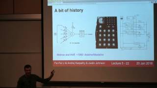
Andrej Karpathy covers activation functions (ReLU, sigmoid, tanh), weight initialization schemes like Kaiming for ReLU, and batch normalization, which normalizes activations and improves gradient flow. He walks through a training workflow: sanity checks, learning-rate bracketing, random hyperparameter search in log-space, and monitoring loss and update scales.
Chapters
How are you guys doing, by the way, with the assignment? Are most of you finished? Anyone finished? Put up your hands. OK, good. So we're doing decent. OK, good. I'll be holding makeup office hours right after this class. Assignment 2 will be released tomorrow or the day after tomorrow. We haven't fully finalized the date. We're still working on it. And we're changing it from last year. And so we're in process of developing it. And we hope to have it as soon as possible. It's meaty but educational. So you do want to get started on it ASAP once it's released. We might be adjusting the due date for assignment 2 because it is slightly larger. And yeah, so we'll be shuffling some of these things around. And also the grading scheme, all of this stuff is kind of just tentative and subject to change because we're still trying to figure out the course. It's still relatively new, and a lot of it is changing. So those are just some heads up items before we start. Now in terms of your project proposal, by the way, which is due in roughly 10 days, I wanted to just bring up a few points because you'll be thinking about your projects and some of you might have some misconceptions about what makes a good or bad project. So just to point out a few of them, the most common one probably is that people are hesitant to work with datasets that are small because they think that ConvNets require a huge amount of data to train. And this is true, there's hundreds of millions of parameters in a ConvNet and they need training. But actually, for your purposes in the project, this is kind of a myth. This is not something you have to worry about a lot. You can work with smaller datasets and it's okay. The reason it's okay is that we have this process that we'll go into in much more detail down the— later in the class called fine-tuning. And the thing is that in practice, you rarely ever train these giant convolutional networks from scratch. You almost always do this pre-training and fine-tuning process. So the way this will work— look like is you almost always take a convolutional network, You train it on some large dataset of, say, images, like, say, on ImageNet, huge amount of data. And then you're interested in some other dataset right there. And you can't train your ConvNet on your small dataset. So we'll train it here, and then we'll transfer it over there. And the way this transfer works like is— so here's a schematic of a convolutional neural network. We start with the image on top, and we'll go through a series of layers down to a classifier. So you're used to this, but we haven't, of course, talked about the specific layers here. But we take that ImageNet, um, pretrained network, we trained on ImageNet, and then we chop off the top layer, the classifier. We chop that off, take it away, and we train the entire convolutional network as a fixed feature extractor. And so you can put that feature extractor on top of your new dataset, and you're just going to swap in a different layer that performs the classification on top. And so depending on how much data you have, you're only going to train the last layer of your convolutional network, or you can do fine-tuning where you actually backpropagate through some portions of the ConvNet. And if you have more data, you're going to do backpropagation deeper through the network. And, uh, in particular, this pre-training step on ImageNet, people do this for you. So there's a huge amount of people who've trained convolutional networks over long periods of time, weeks, on different datasets. And then they upload the weights of the ConvNet online. And so there's something called the Caffe Models Zoo, for example. And these are all these convolutional networks that have been pre-trained on large datasets. They already have lots of the parameters learned. And so you just take this around, then you swap in your dataset, and you fine-tune through the network. So basically, if you don't have a lot of data, that's OK. And you just take a pretrained ConvNet and you just fine-tune it. And so don't be afraid to work with smaller dataset. It's going to work out. OK? The second thing that we saw some problems with last time is that people think they have infinite compute. And this is also a myth I'd just like to point out. Don't be overly ambitious in what you propose. These things take a while to train. You don't have too many GPUs. You're going to have to do hyperparameter optimization. There's a few things you have to worry about here. So we had some projects last year where people proposed projects of training on very large datasets, and you just won't have the time. So be mindful of that. And yeah, you'll get a better sense as we go through the class on what is or is not possible given your compute constraints. OK, so we're going to dive into lectures. Are there any administrative things that I maybe left out that you'd like to ask about? OK, good. So we're going to dive into the material. We have quite a bit of it today. Uh, so just to remind— as a reminder, we're working in this framework of mini-batch stochastic gradient descent for training of neural networks. And basically, it's a 4-step process. Training a neural network is as simple as 1, 2, 3, 4. You sample your data. So a batch of your data from a dataset, you forward it through your network to compute the loss. You backpropagate to compute your gradients, and then you do a parameter update where you tweak your weights slightly in the direction of the gradient. And so when you end up repeating this process, then really what this comes down to is an optimization problem where in the weight space we're converging into areas of the weight space where you have low loss. And that means you're correctly classifying your training set. And we saw that these neural networks can get very large. And I flashed this image of a neural Turing machine. Basically, these are huge computational graphs, and we need to do backpropagation through them. And so we talked about intuitions of backpropagation and the fact that it's really just a recursive application of chain rule from back of the circuit to the front where we're chaining gradients through all the local operations. We looked at looked at some implementations of this concretely with the forward-backward API on both a computational graph and also in terms of its nodes, which also implement the same API and do forward propagation and backward propagation. We looked at specific examples in Torch and Caffe, and I drew this analogy that these are kind of like your Lego blocks. These layers or gates are your Lego blocks from which you build out the entire convolutional networks. Then we talked about neural networks first without the brain stuff, and basically what that amounts to is we're making this F, which goes from your image to class scores, more complex. And then we looked at neural networks from the BrainStuff perspective, where this is a crude analogy of a neuron, and what we're doing is we're stacking these neurons in layers. Okay, so that's roughly what we're doing right now, and we're going to talk in this class about this process of training neural networks effectively. Okay, so we're going to go into that. Before I dive into the details of it, I just wanted to kind of pull out and give you a zoomed out view of a bit of a history of how this field evolved over time. So if you try to find where this field really comes from, when were the first neural networks proposed, and so on, you probably will go back to roughly 1960, where Frank Rosenblatt in 1957 was playing around with something called Perceptron. And the Perceptron basically, it ended up being this implementation in hardware. So they had to, like, they didn't just write code, right? They actually had to build these things up from circuits and electronics, uh, in these times, uh, for the most part. And, um, so basically the perceptron roughly was, uh, this function here. And it looks very similar to what we're familiar with. It's just a wx b. But then the activation function, which we're used to as a sigmoid, that activation function was actually a step function. It was either 1 or 0. It was a binary step function. And so since this is a binary step function, you'll notice that this is non-differentiable operation. So they were not able to backpropagate through this. In fact, the concept of backpropagation for training neural networks had to come much later. And so they came up with these binary stepwise functions, uh, perceptron, and they came up with these learning rules. And so this is an— kind of an ad hoc specified learning rule that tweaked the weights to make the desired outcome from the perceptron match the true— the true, uh, desired values. But there was no concept of a loss function. There was no concept of backpropagation. It's these ad hoc rules which when you look at them, they kind of almost do backprop, but it's kind of funny because of the step function, which is non-differentiable. And then people started to stack these. So in roughly 1960, with the advent of Adeline and Madeline by Widrow and Hoff, they, uh, started to take these perceptron-like things and stack them into the first multi-layer perceptron networks. And, uh, this was still all done in this electronics analogy and actually building it out from hardware. And, uh, but still there's no backpropagation at this time. This was all these rules that they've come up with in terms of, like, thinking about trying to flip bits and seeing if it works better or not. And it was kind of a— there was no view of backpropagation at this time. And so roughly in 1960, people got very excited in building out these circuits, and they thought that, you know, this could go really far. We can have these circuits that learn. You have to remember that back then, the concept of programming was very explicit. You write a series of instructions for a computer. And this is the first time that people are thinking about this kind of data-driven approach where you have some kind of a circuit that can learn. And so this was at the time a huge conceptual leap, um, that people were very excited about. Unfortunately, these networks would not actually end up working very well right away. So in terms of 1960, for example, they got slightly overexcited and overpromised and then slightly underdelivered. And so throughout the period of 1970s, actually the field of neural networks was very quiet. And not much research has been done. The next boost actually came about roughly in 1986. And in 1986, people— there was this influential paper that basically is the first time that you see backpropagation-like rules in a nicely presented format. And so this is Rumelhart, Hinton, and Wilson. And they were playing with multilayer perceptrons. And this is the first time when you go to the paper where you actually see something that looks like backpropagation. And so at this point, they already discarded this idea of ad hoc rules, and they formulated the loss function and talked about backpropagation and gradient descent and so on. And so at this time, people got excited again in 1986 because they felt that they now had a principled, nice credit assignment kind of scheme by backpropagation, and they could train multilayer networks. The problem, unfortunately, was that when they tried to scale up these networks to make them deeper or larger, they didn't work very well compared to some of the other things that might be in your machine learning toolkits. And so they just did not give very good results at this time. And, uh, training would get stuck and backpropagation was basically not working very well, especially if you wanted to have large deep networks. And this was the case for actually roughly 20 years where again there was less research on neural networks because somehow it wasn't working very well enough and you couldn't train deep nets. And in 2006, the research was, uh, research was again reinvigorated with a paper in Science by Hinton Andrej Karpathy and Ruslan Selakutdinov. Selakutdinov. I can't say his name. Sorry. But basically what they found here was this was roughly the first time where you can actually have, like, say, a 10-layer neural network that trains properly. And what they did was instead of training all the layers, like 10 layers, by backpropagation at a single pass, they came up with this unsupervised pre-training scheme using what's called restricted Boltzmann machine. And so what this amounts to is you train your first layer using an unsupervised objective. And then you train your second layer on top of it, and then third, and fourth, and so on. And then once all of these are trained, then you put them all together, and then you start backpropagation. Then you start the fine-tuning step. So it was a two-step process of first we do this pre-training stepwise through the layers, and then we plug them in, and then backpropagation works. And so this was the first time where backpropagation— it needed basically this initialization from the unsupervised pre-training, otherwise it would not work out of, like, from scratch. And we're going to see why in this lecture, it's kind of tricky to get these deep networks to train from scratch using just backprop. And you have to really think about it. And so it turned out later that you actually don't need this unsupervised process. You can just train with backprop right away. But you have to be very careful with initialization. And they used sigmoid networks at this point. And sigmoids are just not a great activation function to use. And so basically, backprop works, but you have to be careful in how you use it. And so this was in 2006. So a bit more researchers kind of came back to the area. And it was rebranded as deep learning, but really, it's still neural networks, uh, synonymous, but it's a better word for, uh, PR. And, um, so basically at this point, uh, things started to work relatively well and people could actually train these deeper networks. Now, still not too many people paid attention. And when people started to really pay attention was roughly, I think, around 2010 and 2012. So specifically in 2010, there were the first really big results where neural networks really worked really well compared to everything else that you had in your machine learning toolkit, like say, uh, kernels or SVMs and so on. And this was specifically in the speech recognition area where they took this GMM-HMM framework and they swapped out one part and subbed in a neural network. And that neural network gave them huge improvements in 2010. And this was work done in Microsoft. And so people started to pay attention because this was the first time neural networks really gave large improvements. And then we saw that again in 2012 where it played out even more dramatically. In, uh, in the domain of visual recognition in computer vision, where basically we took, uh, this 2012, um, uh, network by Alex Kruchevsky, Ilya Sutskever, and Geoff Hinton, and basically it crushed all the competition from all the features, and there was a really large, um, improvement from these neural networks, um, that we witnessed, and that's when people really started to pay attention, and that's— since then, the field has kind of exploded. And there's a lot of area done in this field now. And so we'll go into details, I think, a bit later in the class on why it started to work really in 2010. It's a combination of things, but I think it's— we got— we figured out better ways of initializing, of getting these things to work, of activation functions. And we had GPUs, and we had much more data. And so really, a lot of the stuff before didn't quite work because it was just not there in terms of compute data. And some of the ideas just needed tweaking. Okay, and so that's rough historical setting. So we basically went through over-promising, under-delivering, over-promising, under-delivering, and now it seems like things are actually starting to work really well, and so that's where we are at this point. Okay, so I'm going to now dive into the specifics, and we'll see exactly— we'll actually dive into neural networks and how you train them properly. So the overview of what we're going to cover over the course of the next two lectures is a whole bunch of independent things. So I'll just be kind of peppering you with all these little areas that we have to understand and see what people do in each case. And we'll go through them, the pros and cons of all choices, how you actually properly train these neural networks in real-world datasets. So the first thing we're going to talk about is activation functions, as I promised, I think, a lecture or so ago. So activation function is this function f at the top of neuron, and we saw that it can have many different forms. So sigmoid, tanh, ReLU, these are all different proposals for what these activation functions can look like. And we're going to go through some pros and cons in how you think about what an activation— what are good desirable properties of an activation function. So historically, the one that has been used the most is the sigmoid nonlinearity, which looks like this. So it's basically a squashing function. It takes a real-valued number, squashes it to be between 0 and 1. And so the first problem with the sigmoid is that, as was pointed out a few lectures ago, um, there's a problem that saturated neurons, which are neurons that output either very close to 0 or very close to 1, those neurons kill gradients during backpropagation. And so I'd like to expand on this and show you exactly what this means. Uh, and this contributes to something that we'll go into called the vanishing gradient problem. So let's look at a sigmoid gate. In the back— in the circuit. It receives some value x, and sigma of x comes out. And then in backprop, we have dl by d sigma, and we'd like to backprop it through the sigmoid gate to using chain rule so that we have dl by dx at the end. And you can see that through chain rule basically tells us to multiply those two quantities. And so think about what happens when this sigmoid gate receives input of either -10 or 0 or 10. It computes some value, and then it's getting some gradient from the top, And what happens to that gradient as you backprop through the circuit in any of these cases? What is the possible problem in some of these cases? The gradient is really low when x is -10 or 10. So, uh, okay. So you're saying that the gradient is very low when x is -10 or 10. And the way to see this is basically, we have this local gradient here that will be multiplying with this gradient. This local gradient d phi— d sigma by dx. When you're at negative 10, you can see that the gradient is basically 0 because the slope at this point is 0. And gradient at 10 will also be near 0. And so the issue is that your gradient will drop in from here, but if your neuron is saturated, so it basically either outputted 0 or it outputted 1, then the gradient will be killed. It'll just be multiplied by a very tiny number, and gradient flow will stop through the, through the sigmoid neuron. So you can imagine if you have a large network of sigmoid neurons and many of them are in a saturated regime where they're either 0 or 1, then gradients can't backpropagate through the network because they'll be stopped if your sigmoid neurons are in these saturated regimes. Gradients only flow if you're kind of in a safer zone in what we call an active region of a sigmoid. And so that's kind of a problem. We'll see a bit more about this soon. Another problem with sigmoids is that their outputs are not zero-centered. So we'll talk about data preprocessing soon, but you always want to— when you preprocess your data, you want to make sure that it's zero-centered, right? And in this case, suppose you have a big network of several layers of sigmoid neurons. They're outputting these non-zero-centered values between 0 and 1, and we're putting more basically linear classifiers that were stacking on top of each other. And the problem roughly with non-zero centered outputs, I'll just try to give you a bit of an intuition on what goes wrong. Um, so consider a neuron that computes this function, right? So it's a sigmoid neuron looking at, um, it's just computing wx b. And what can we say about— think about what you can say about the gradients on w during backpropagation if your x's are all positive, in this case between 0 and 1. So maybe you're a neuron somewhere deep in the network. What can you say about the weights if all the x's are positive numbers? They're kind of constrained in a way. Go ahead. All the elements of the gradient of w is positive or negative. Right. So what you said is all the gradients of w are either all positive or all negative. And that is because gradient flows in from the top. And if you think about the expression for all the w gradients, they're basically x times the gradient on f. And so if the gradient of— on— at the output of the neuron is positive, then all your w gradients will be positive and vice versa. So basically you end up with this case where suppose you have just two weights. So you have the first weight and the second weight. What ends up happening is either all your gradient for that— for that as this, as this input goes through and you compute your gradient in the weights, they're either all positive or they're all negative. And so the issue is that you're constrained in the kind of update you can make, and you end up with this undesirable zigzagging path if you want to get to some parts that are outside of these regions. So this is kind of like a slightly hand-wavy reason here. Um, but just to give you intuition, and you can see this empirically when you train with things that are not zero-centered, you'll observe slower convergence. And this is a bit of a hand-wavy reason for why that might happen. But I think, um, if you actually wanted to go much deeper into that, you can, and there are papers written about this. But you have to then reason about, uh, mathematics of Fisher matrices and natural gradients, and it gets a bit more complex than this. But I just wanted to give you intuition for you want to have zero-centered things in the input, you want to have zero-centered things throughout, otherwise things, things don't converge as nicely. And so that is a downside of a sigmoid neuron. The last one is that exp function inside this expression is kind of expensive to compute compared to some of the alternatives of other nonlinearities. So it's just a small detail, I suppose. When you actually train these large convolutional networks, most of the compute time is in convolutions and these dot products. It's not in this exp operation. So it's kind of vanishingly small contribution, but it's still something that is a bit of a downside compared to the other parts. So I'll go into tanh, and I'll ask a few— I'll take a few questions then. So tanh is an attempt to fix one of these problems, in particular, the fact that it's non-zero-centered sigmoid. So, um, Ian LeCun in 1991 wrote a very nice, uh, paper on how you optimize neural networks, and I've linked to it from the syllabus. And he recommended that people use, uh, tanh(x) instead of sigmoid. And tanh(x) basically is kind of like two sigmoids put together. You end up with, uh, being between -1 and 1, and so your outputs are zero-centered. Uh, but otherwise you have still some, some of the other problems. Like for example, you have these regions where if your neurons get saturated, no gradients flow, and so we haven't really fixed that at this point. Um, but so tanh is, I think, strictly preferred to sigmoid because it has all the same problems except for one. Okay. Um, I'll continue and then maybe we can take more questions. So around 2012, in a paper by Alex Kruchevskyi— this is the first convolutional networks paper— they proposed that actually they noticed that this nonlinearity where you use max of 0 and x instead of sigmoid or tanh just makes your networks converge much quicker. And in their experiments, almost by a factor of 6. And so we can go back and try to think about why is this. And we're kind of reading into it. Like, you can see that it works better in practice, but explaining it is not always as easy. So here's some hand-wavy reasons, I think, for why people are thinking that, uh, this works much better. So one thing is that this, um, this ReLU neuron, it does not saturate, at least in the positive region. So at least in this region, you don't have this vanishing gradient problem where your gradients will just kind of die, and you have this, uh, issue where the neurons are only active in a small area that is bounded from both sides, but these neurons are actually active in a sense that they backpropagate correctly, or not correctly, but at least they don't not backpropagate all zeros, at least in half of their regions. They're much more computationally efficient because doing— you're just doing thresholding. And experimentally, you can see that this converges much, much faster. So this is called the ReLU neuron, or the rectified linear unit, and it was pointed out in this paper for the first time that this works much better. And this is kind of like the default recommendation of what you should use at this point. At the same time, there are several problems with this ReLU neuron. So one thing, again, notice that it's not zero-centered outputs, so not completely ideal perhaps. And a slight annoyance of the ReLU neuron that we can talk about and think about is what happens when this ReLU neuron outputs a 0? What happens during backpropagation if a ReLU neuron does not become active? So in the forward pass, a ReLU neuron stays inactive, then during backprop, what does it do? [Speaker:AUDIENCE] It kills the gradient. It kills, right, it kills the gradient. And so the way to see this, of course, is that we have the same picture. And if you're at negative, say, 10, then your local gradient here will just be 0 because there's no— there's just 0 gradient identically. It's not just you squish the gradient down, you actually kill it completely. So any neuron that does not activate will not backpropagate downwards, its weights will not be updated, and nothing happens below it, at least for its contribution. And at x equals 10, what is the local gradient? It's just 1. So a ReLU neuron just passes through gradients, just a gate. If during the forward pass its output was positive, then it just passes gradients through. Otherwise, it kills it. It's kind of like a gradient gate. And by the way, what happens when x is 0? What is your gradient at that point? Questionable. [Speaker:AUDIENCE] Undefined. [Speaker:ANDREJ KARPATHY] It's actually undefined. That's right. The gradient does not exist at that point. We only talk about— whenever I talk about gradient, just assume that I always mean subgradient, which is a generalization of gradients to functions that are sometimes non-differentiable. So here, the limit does not exist. But there's a whole bunch of subgradients that could be 0 or 1. And so that's what we use usually. In practice, this distinction doesn't really matter too much. But I wanted to also point this out in the case of the binary max gate, max of x and y. And someone asked the question, what happens if x and y are equal? Then in that case, you kind of also have a kink in the function and makes it non-differentiable. But in practice, these things don't really matter. Just pick one. So you can have a gradient of 0 or 1 there, and things will work just fine. And that's roughly because these are very unlikely cases that you end up right there. OK, so the issue with ReLU— roughly. Here's the problem that happens in practice. You try to use ReLU units, and one thing that you have to be aware of is you have these neurons that if they don't output anything, they won't get any gradient. They'll kill it, and they won't update. And so let's see. So the issue is suppose you have a— sometimes what can happen is when you initialize your ReLU neurons, you can initialize them in a non— not very, um, lucky way. And what ends up happening is, suppose this is your data cloud of inputs to your ReLU neurons. What you can end up with is a— what we call a dead ReLU, a dead ReLU neuron. So if this neuron only activates in a region, uh, outside of your data cloud, then this dead ReLU will never become activated, and then it will never update. And so this can happen in one of two ways. Either during initialization you were really, really unlucky and you happened to sample weights for the reLU neuron in such a way that that neuron will never turn on. In that case, the neuron will not train. But more often what happens is during training, if your learning rate is high, then think about these neurons as kind of like jittering around. And what can happen sometimes by chance is they just get knocked off the data manifold. And when that happens, then they will never get activated again, and they, they will not come back to the data manifold. And you can see this actually in practice. Like, sometimes you can train a big, uh, neural net with ReLU units, and you train it, and it seems to work fine. And then what you do, you stop the training, and you pass your entire training dataset through your network, and you look at the statistics of every single neuron. And what, what, what can happen is that as much as like 10 or 20% of your network is dead. They— these are neurons that never turned on for anything in the training data. And this can actually happen. Usually it's, uh, because your learning rate was high, and so those are just like dead parts of your network. and, uh, you can come up with hacky schemes for reinitializing these things and so on. People don't, uh, usually, uh, do it as much, but that's something to be aware of, and, uh, it's a problem with this nonlinearity. And, uh, so especially for initialization, because of this dead ReLU problem, what people like to do is normally you initialize the biases with 0. Instead, people initialize with slightly positive numbers like, say, 0.01, because that makes it more likely that at initialization these ReLU neurons will output positive numbers and they'll get updates. So it makes it less likely that the neuron will just never become activated ever throughout training. But I don't actually— I think this is slightly of a controversial point. I've seen people claim that it helps. I've seen some people say that it actually doesn't help at all. And so just something to think about. Okay, any questions at this point? We had sigmoid, tanh, and ReLU. I'm going to go into some other ones. Okay, good. So let's look at things like people trying to fix ReLUs. So one issue with ReLUs is these dead neurons are not ideal. So here's one proposal, which is called the Leaky ReLU. And the idea with Leaky ReLU is basically we want this kink, and we want this piecewise linearity, and we want this efficiency of ReLU. But the issue is that in these— this region, your gradients die. So instead, let's make this slightly negatively sloped here. —or slightly positively sloped, I suppose—in this region. And so you end up with this function, and that's called a leaky ReLU. And so some people— there are papers showing that this works slightly better. You don't have this issue of neurons dying. But I think it's not completely established that this works always better. And then some people play with this even more. So right now this is 0.01, but that can actually be an arbitrary parameter. And then you get something that's called a parametric rectifier, or PReLU. Basically, the idea here is you introduce— this is 0.01, that can be an arbitrary alpha, which is a parameter in your network, and this alpha can be learned. You can backpropagate into it. So these neurons basically can choose what slope to have in this negative region. So they can become a ReLU if they want to, or they can become a leaky ReLU, or they can be— they have the choice roughly for every neuron. So this is the kinds of things that people play with when they try to design better nonlinearities. Good. So you're saying that alpha can be set by neurons above stream? Um, so alpha here would be a parameter that you backpropagate to in just a very normal way. In your computational graph, there's— every neuron will have its alpha, just like it has its own bias. Okay. Go ahead. Is there some restriction on the, uh, activation function? Can alpha be 1? Yeah, I'm not sure if they worry about this a lot. So if alpha is 1, then you're going to get an identity. So that's probably not something that backpropagation will want in the sense that if that was an identity, then that shouldn't be very computationally useful. So you might expect that maybe backpropagation should not actually get you to those regions of the space, hand-wavy reason perhaps. I don't actually think— if I remember correctly, there's no specific things where people really worry about that too much. But I could be wrong. I read the paper a while ago now, and I don't use these too much in my own work. Okay, and then so one issue still is, as we saw, so these are different schemes for fixing the, the dead ReLU neurons. There's another paper that only came out, for example, roughly 2 months ago. So this just gives you a sense of how new this field is. There are papers coming out just 2 months ago trying to propose new activation functions. One of them is exponential linear units, or ELU. So just to give you an idea about what people play with, it tries to have all the benefits of ReLU, but it tries to get rid of this downside of being non-zero centered. And so what they end up with is this blue function here that looks like a ReLU, but in the negative region, it doesn't just go to zero or it doesn't just go down as a leaky ReLU, but it has this funny shape. And there are two pages of math in that paper justifying partly why you want that. And roughly when you do this, then you end up with zero mean outputs. And they claim that this trains better. And I think there's some controversy about this and And so we're basically trying to figure all of this out, active area of research, and we're not sure what to do yet. But ReLUs right now are like a safe recommendation if you're careful with it. Okay, so that's ELUs. And one more I would like to note, mention, because it's relatively common and you'll see it if you read about neural networks, is this MaxEnt neuron from Ian Goodfellow et al. And basically it's a very different form of a neuron. It's not just an activation function that looks different, it actually changes what a neuron computes or how it computes. So it doesn't just have this form of f of w transpose x, it actually has two weights, and then it computes max of w transpose x plus b and another set of w transpose x plus b. So you end up with these, like, two hyperplanes that you take a max over, and that's what the neuron computes. So you can see that there are many ways of playing with these activation functions. Uh, so this doesn't have some of the downsides of, of a ReLU. This won't die, and it's still piecewise linear, it's still efficient, But, uh, now every single neuron has two weights, and so you've kind of doubled the number of parameters per neuron, and so maybe that's not as ideal. So some people, uh, use this, but I think it's, uh, it's not super common. I would say that ReLUs are still most common. Go ahead. Because the loss functions will be different when we use different activation functions, the weights which you obtain might not be the same, right? Even if— I mean, they might have different convergence rates, but they also can result in different weights, right? At the end of the simulation. Uh, that's right. So what is your question? Sorry. Because the loss functions themselves are different when you use different activation functions, so the weights also will be different in both if you use different activation functions, right? Uh, that's right. So the weights will end up, uh, yeah, based on what the activation functions are, the dynamics of the backprop into those weights will be different, and so you end up with different weights, for sure. So, uh, isn't the argument more like which loss function is like, uh, closer to the reality, which loss function is better in some sense? [Speaker:ANDREJ KARPATHY] Yeah, I think it's complicated. The reason it's complicated is a lot of the optimization process is not just about the loss function, but just like about the dynamics of the backward flow of gradients. And we'll see a bit about that in the next few slides. You have to really think about it dynamically more than just loss landscape and how— so it's a complex— and also we use specifically stochastic gradient descent and it has a particular form and some things play nicer, some nonlinearities play nicer with the fact, like the optimization is tied, the update is tied into all of this as well and it's kind of all interacting together and the choice of, um, these activation functions and the choice of your updates are kind of coupled and it's kind of very unclear when you actually optimize this kind of complex thing. So TL;DR here is that use ReLU. You can try out these guys. You can try out tanh, but you shouldn't expect too much. I don't think people use it too much right now. And don't use sigmoid because basically tanh is strictly better, and you won't see people use sigmoid now anymore. Of course, we use it in things like long short-term memory units, LSTMs, and so on. And we'll go into that in a bit in recurrent neural networks. But there are specific reasons why we use them there and that we'll see later in the class. And they are— they're used differently than what we have covered so far in like this just fully connected sandwich of matrix multiply, nonlinearity, and so on, just having a basic neural network. Okay, so that's everything I wanted to say about activation functions. It's basically this one hyperparameter in our functions that we worry about. There's research about it, and we haven't fully figured it out, and there's some pros and cons, and many of them come down to thinking about how the gradient flows through your network. And these issues like dead ReLUs, and you have to really know about the gradient flow if you try to debug your networks and to understand what's going on. Okay? So let's look at data preprocessing very briefly. Uh, how am I on time? Okay. So data preprocessing, just very briefly. Normally, suppose you just have a cloud of original data in two dimensions here. Very common to zero-center your data. So that just means that along every single feature, we subtract the mean. People sometimes also, when you go through machine learning literature, try to normalize the data. So in every single dimension, you normalize, say, by standard deviation, called standardizing. Or you can make sure that the min and the max are within, say, -1 or 1, and so on. There are several schemes for doing so. In images, it's not as common because you don't have separate different features that could be at different units. Everything is just pixels, and they're all bounded between 0 and 255. So it's not as common to normalize the data, but it's very common to zero-center your data. You can go further. Normally in machine learning, you can, uh, go ahead and your data has some covariance structure by default. You can go ahead and make that covariance structure be diagonal, say for example by applying PCA. Or you can go even further and you can whiten your data. And what that means is you kind of even squish— after you've performed PCA, you also squish your data so that your covariance matrix becomes just a diagonal. And so that's another form of preprocessing you might see people, um, talk about. And these are both— I go much more detail in the class notes on these. I don't want to go into too many details on them because it turns out that in images we don't actually end up using these even though they're common in machine learning. So in images specifically, what's common is just the mean centering and then a particular variant of mean centering that is slightly more convenient in practice. So in mean centering, we say have 32 by 32 by 3 images of CIFAR. If you want to center your data, then for every single pixel, you compute its mean value over the training set, and you subtract that out. So what you end up with is this mean image that has basically a dimension of 32 by 32 by 3. So I think the mean image, for example, for ImageNet is just this, uh, orange blob. So you end up subtracting that from every single image to center your data, uh, to have better training dynamics. And, uh, one other form that is slightly more convenient is, uh, subtracting just a per-channel mean. So you go in red, green, and blue channel, and you compute to the mean across all of space. So you just end up with basically 3 numbers of the means in red, green, and blue channel, and you subtract those out. And so some networks, uh, use that instead. So those are the 2 common schemes. Uh, this one is slightly more convenient because you only have to worry about those 3 numbers. You don't have to worry about a giant array of mean image that you have to ship around everywhere when you're actually coding this up. Okay? So not too much, uh, more I want to say about this. Um, just, uh, basically subtract the mean in computer vision applications. Things don't get much more complex than that. In particular, doing PCA and so on, this used to be slightly common. The issue is you can't apply it on full images because your images are very high-dimensional objects with lots of pixels. And so these, uh, covariance matrices would be huge. And people try to do things like only doing whitening locally. So you would slide a whitening filter through your images spatially. And that used to be done several years ago, but it's not as common now. It doesn't seem to matter too much. Okay, good. So we'll dive into weight initialization. Uh, very, very important topic. One of the reasons that I think early neural networks didn't quite work as well is because people are just not careful enough with this. So one of the first things we can look at is, first of all, how not to do weight initialization. So in particular, you might be tempted to just say, okay, let's start off at all the weights are equal to 0, and you use that in your neural network. So suppose you have like a 10-layer neural network and you set all the weights to 0. Why doesn't that work? Why isn't that a good idea? [Speaker:AUDIENCE] All data will output the same? [Speaker:ANDREJ KARPATHY] Sorry, go ahead. [Speaker:AUDIENCE] All output will just all output 0. [Speaker:ANDREJ KARPATHY] Yeah, so basically just all your neurons output the same thing. In backprop, they will behave the same way. And so there's nothing, as we like to call it, symmetry breaking. So all the neurons are computing the same stuff. And so in backprop, they will all look the same. They'll compute the same gradients and so on. So not the best thing. So instead, people use small numbers, small random numbers. So one way you can do that, for example, that is a relatively common thing to do, is you sample from a unit Gaussian with, uh, 0.01 standard deviation. So small random numbers. Um, so that's your W matrix, how you would initialize it. Now, the issue with this initialization is that it works okay, but you'll find that it only works okay if you have small networks. But as you start to go deeper and deeper, with neural networks, you have to be much more careful about initialization. And I'd like to go into exactly what breaks and how it breaks and why it breaks when you try to do these naive initialization strategies and you try to have deep networks. So let's look at what goes wrong. Um, so what I've written here is a small IPython notebook. Uh, so what we're doing here is— I'm going to step through this just briefly. Um, I'm sampling a dataset of 1,000 points that are 500-dimensional. And then I'm creating a whole bunch of hidden layers and nonlinearities. So say right now we have 10 layers of 500 units, and we're using tanh. Um, and then what I'm doing here is I'm just, um, basically taking unit Gaussian data, and I'm forwarding it through the network. And with this particular initialization strategy, where right now that initialization strategy is what I described in the previous slide. So you sample from unit Gaussian and you scale it by 0.01. So what I'm doing here in this for loop is I'm forward propagating this network, which is right now made up of just a series of, uh, layers of the same size. So we have 10 layers of 500 neurons on each layer, and I'm forward propagating with this initialization strategy for a unit Gaussian data. And what we— I want to look at is what happens to the statistics of the hidden— of the, um, neurons activations throughout the network with this initialization. So we're going to look specifically at the mean and the standard deviation and we're going to plot the mean standard deviation, and we're going to plot the histograms. So we take all this data through, and then say at the 5th layer, we're going to look at what the— what values the neurons take on in, say, the 5th or 6th or 7th layer, and we're going to make histograms of those. So with this initialization, if you run this experiment, you end up— it ends up looking as follows. So here I'm printing it out. We start off with a mean of 0 and standard deviation of 1. That's our data. And now I'm forward propagating, and as I go to the 10th layer, look at what happens to the mean. We're using tanh, so tanh is symmetric. So as you might expect, the mean stays around 0, but the standard deviation, look at what happens to it. It started off at 1, and suddenly the standard deviation goes to 0.2, then 0.04, and it just plummets down to 0. So the standard deviation of these neurons just goes down to 0. Looking at the histograms here at every single layer, At the first layer, the histogram is reasonable. So we have a spread of numbers between -1 and 1. And then what ends up happening to it, this just collapses to a tight distribution at exactly 0. So what ends up happening with this initialization for this 10-layer network is all the 10H neurons just end up outputting just 0. So at the last layer, these are tiny numbers of like near 0 values. And so all activations basically become 0. And why is this an issue? Okay. So think about what happens to the dynamics of the backward pass to the gradients. When you have tiny numbers in the activations, your x's are tiny numbers on the last few layers. What do these gradients look like on the weights in these layers and what happens to the backward pass? So first of all, suppose my— so there is a layer here that looks at some layer before it, and almost all the inputs are tiny numbers. That's the x. x is a tiny number. What is the gradient? What might you expect the gradients for the w to be in that case for those layers? Very small. Sorry, you said very small? Yeah. So why would they be very small? x is a— Uh, that's right. So the gradient for W will be equal to X times the gradient from the top. Okay. And so if X are tiny numbers, then your gradients for W are tiny numbers as well. And so these guys will basically have almost no gradient accumulated. Now we can also look at what happens, um, with these matrices again. We, we took, um, data that was distributed as a unit Gaussian, and the beginning, and then we ended up multiplying it by w and activation function, and we saw that basically everything goes to zero. This just collapses over time. And think about the backward pass as we chain the gradient through these layers in backpropagation. What we're doing effectively is some of the gradient kind of forks off into our gradient w, and we saw that those are tiny numbers. But then through backpropagation, we're going through gradients of x. And so what we end up doing when we backprop through here is we again end up multiplying by W again and again at every single layer. And if you take unit Gaussian data and you multiply it by Ws at this scale, you can see that everything goes to zero. And the same thing will happen in backward pass. We're successively multiplying by W as we backpropagate into X on every single layer. And we're— as we do that, this gradient which started off with reasonable numbers from your loss function will end up just going towards zero as you keep doing this process. And you end up with gradients here that are basically just tiny, tiny numbers. And so you basically end up with very, very low gradients throughout this network because of this reason. And this is something that we refer to as vanishing gradient. As this gradient travels through, with this particular initialization, you can see that the magnitude of the gradient will just go down when we used this initialization for W of 1e-2. Okay? So we can try a different extreme. Instead of scaling here as we scaled with 1e-2, we can try a different scale of the W matrix at initialization. So suppose I try 1.0 instead of 0.01. We'll see another funny thing happen because now we've overshot the other way in a sense that you can see that, uh, well, maybe it's best to look at, um, the distributions here. You can see that everything is completely saturated. These tanh neurons are either all -1 or all 1. 1. I mean, the distribution is really just everything is supersaturated. Your entire network, all the neurons throughout the network are either -1 or 1 because the weights are too large and they keep oversaturating the tanh neurons because the scores that end up going through the nonlinearity are just very large because the weights are large. And so everything is supersaturated. So what are the gradients flowing through your network? It's just terrible. It's a complete disaster, right? It's just zeros for every— just— exponentially zero, and you die. So you can train for a very long time, and what you'll see when this happens is your loss is just not moving at all because nothing is backpropagating because all the neurons are saturated and nothing is being updated. Okay? So this initialization, as you might expect, actually is like super tricky to set, and it needs to be kind of— in this particular case, it needs to be somewhere between 1 and 0.01. Okay? And so you can be slightly more principled instead of trying different values, and there are some papers written on this. So for example, in 2010, um, there was a proposal for what we now call the Xavier initialization from Glorot et al. And they kind of, um, went through and they looked at the expression for the variance of your neurons. And you can write this out, and you can basically propose a specific initialization strategy for how you scale your gradients. So I don't have to try 0.01, I don't have to try 1 or whatever else. Uh, so they recommend this kind of initialization where you divide by the square root of the number of inputs for every single neuron. So if you have lots of inputs, then you end up with lower weights. And intuitively that makes sense because you're doing more weight— you have more stuff that goes into your weighted sum. So you want less of an interaction to all of them. And if you have smaller number of, uh, units that are feeding into your layer, then you want larger weights because then there's only a few of them and you want to have a variance of 1. Andrej Karpathy. Um, so just to back up a bit, the idea here is they were looking at a single neuron, no activation functions included, it's just a linear neuron. And all they're saying is if you want— if you're getting unit Gaussian data as input and you'd like this linear neuron to have a variance of 1, then you should initialize your weights with this amount. And in the notes, I go into exactly how this is derived. It's just, uh, some math with standard deviations. And basically, uh, this is a reasonable initialization. So I can use that instead. And you can see that if I use it here, the distributions end up being more sensible. So we're again looking at the histogram between -1 and 1 of these 10 H units. And you get a more sensible number here. And you actually have— you're within the active region of all these 10 H's. And so you can expect that this will be a much better initialization because things are in the active regions and things will train from the start. Nothing is supersaturated in the beginning. The reason that this doesn't just end up being very nice and the reason we still have convergence down here is because this paper doesn't take into account the nonlinearities, in this case the tanh. And so the tanh nonlinearity ends up like kind of deforming your statistics of the variance throughout. And so if you stack this up, it ends up still, you know, doing something to distribution. In this case, it seems that the standard deviation goes down, but it's not as dramatic as if you were to set this by just trial and error. And so this is like a reasonable initialization, uh, to, to use in your neural networks compared to just setting it to 0.01. And so people end up using this in practice, uh, sometimes. But so this works in the case of tanh does something reasonable. It turns out if you try to put it into a rectified linear unit network, it doesn't work as well. And the decrease in the standard deviations will be much more rapid. So looking at a ReLU neuron, in the first layer, it has some distribution. And then this distribution, as you can see, just gets more and more peaky at 0. So more and more neurons are, are not activating with this initialization. So using the Xavier initialization in a rectified layer, uh, layer net does not do good things. And so again, thinking about this paper, they don't actually talk about nonlinearities and the ReLU neurons, they compute this weighted sum, which is within their domain here, But now after the weighted sum, you do a ReLU. So you kill half of the distribution, you set it to 0. And intuitively what that does to your distribution of your outputs is it basically halves your variance. And so it turns out, um, as was proposed in this paper just last year in fact, someone said basically, um, look, there's a factor of 2 you're not accounting for because these ReLU neurons, they effectively half your variance each time because you take everything— like say you have unit Gaussian inputs, You take them through your nonlinearity, you have unit Gaussian stuff out, but now you ReLU that, and so you end up having the variance. So you need to account for it with an extra 2. And when you do that, then you get proper distributions specifically for the ReLU neuron. And so in this initialization, where if you're using ReLU nets, you have to worry about that extra factor of 2, and everything will come out nicely. And you won't get this factor of 2 that keeps building up, and it screws up your activations exponentially. Okay? So basically this is tricky, tricky stuff, and it really matters in practice. In practice, in their paper for example, they compare having the factor of 2 or not having that factor of 2. And it matters when you have really deep networks. In this case, I think they had a few dozen layers. If you account for the factor of 2, you converge. If you don't account for that factor of 2, you does nothing. It's just zero loss. Okay? So very important stuff. Uh, you need— really need to think it through. You have to be careful with initialization. If it's incorrectly set, bad things happen. And so specifically in the case if you have neural networks with ReLU units, there's a correct answer to use, and that's this initialization from Kaiming. So tricky stuff. This is partly why neural networks didn't work for a long time, is we just— I think people didn't fully maybe appreciate just how difficult this was to get right. Tricky. And so I just like to point out that proper initialization, basically active area of research. You can see that papers are still being published on this. A large number of, uh, papers just proposing different ways of initializing your networks. Uh, these last few are interesting as well because they don't give you a formula for initializing. They have these data-driven ways of initializing the networks. And so you take a batch of data, you forward it through your network, which is now an arbitrary network, and you look at the variances at every single point in your network. And intuitively, you don't want your variances to go to 0. You don't want them to explode. You want everything to have roughly, say, like, be a unit Gaussian throughout your network. And so they iteratively scale these weights in your network so that you have roughly unit Gaussian activations everywhere, or on the order of that, basically. And so there are some data-driven techniques and a line of work on how to properly initialize. OK, so I'm going to go into some— I'm going to go into a technique that alleviates a lot of these problems. But right now, I could take some questions if there are any at this point. Go ahead. [Speaker:AUDIENCE] Would it make any sense to standardize the gradient coming in by dividing the variance or something? [Speaker:ANDREJ KARPATHY] Would it make sense to standardize the gradient coming in by dividing by the variance? Possibly, but then you're not doing backpropagation. Because if you meddle with the gradient, then it's not clear what your objective is anymore. And so you're not getting necessarily gradient. So that's maybe the only concern. I'm not sure what would happen. You can try to normalize the gradient. I think the method I'm going to propose in a bit is actually doing something to the effect of that, but in a clean way. OK? Cool. So let's go into something that actually fixes a lot of these problems in practice. It's called batch normalization, and it was only proposed last year. And so I couldn't even cover this last year in this class, but now I can. So this actually helps a lot. OK? The basic idea in batch normalization paper is, okay, you want roughly unit Gaussian activations in every single part of your network. And so just, just do that. Just, just make them unit Gaussian. Okay, you can do that because making something unit Gaussian is a completely differentiable function. And so it's okay, you can backpropagate through it. And so what they do is you're taking a mini-batch of your data and you're taking it through your network. We're going to be inserting these batch normalization layers into your network. And the batch normalization layers, they take your input x, and they make sure that in every single feature dimension across the batch, you have unit Gaussian activations. So say you have a batch of 100 examples going through the network. Uh, maybe this is a good example here. So you have a batch of activations. So you have n things in your mini-batch, and you have d features or d activations of neurons, uh, that are at some po— some part, and this is an input to your batch normalization layer. So this is a matrix of X of activations. And batch normalization effectively, it, um, evaluates the empirical mean and variance along every single feature, and it just divides by it. So whatever your X was, it just makes sure that every single column here has unit— is a unit Gaussian. And so that's a perfectly differentiable function, and it just applies it at every single feature or activation independently across the batch. Okay? So you can do that. And that's a— that turns out to be a very good idea. Now, one problem with this scheme— so this is the way this will work is we'll have— normally we have fully connected followed by nonlinearity, fully connected followed by nonlinearity, and we have a deep network of this. Now we're going to be inserting these batch normalization layers right after fully connected layers. Or equivalently after convolutional layers, as we'll see soon with convolutional networks. And basically, we insert them there, and they make sure that everything is roughly unit Gaussian at every single step of the network because we just make it so. And, um, one problem you might think of with this— with this is that that seems like an unnecessary constraint. So when you put a batch normalization here after fully connected, the outputs will definitely be unit Gaussian because you normalize them. But it's not clear that tanh actually wants to receive unit Gaussian inputs. So if you think about the form of tanh, it has a specific scale to it. It's not clear that a neural network wants to have this hard constraint of making sure that, uh, batch norm outputs are exactly unit Gaussian before the tanh. Uh, because you— if you'd like the network to pick if it wants your tanh outputs to be more or less diffuse, more or less saturated, and right now it wouldn't be able to do that. So a small patch on top of it, this is the second part of batch normalization, is not only do you normalize x, but after normalization you allow the network to shift by gamma and add a b for every single feature input. And so what this allows the network to do, and these are all parameters, so gamma and b here are parameters that we're going to backprop, uh, backprop into, and, uh, they just, um, allow the network to, to shift After you've normalized to unit Gaussian, they allow this bump to shift and scale if the network wants to. And so we initialize, though, presumably with 1 and 0 or something like that. And then we can— the network can choose to adjust them. And by adjusting these, you can imagine that once we feed into tanh, the network can choose through the backdrop signal to make the tanh more or less peaky or saturated in whatever way it wants. But you're not going to get into this trouble where things just completely die or explode in the beginning of optimization. And so things will train right away, and then backpropagation can take over and can fine-tune it over time. And note one more important feature, by the way, is that, um, if you set these gamma and b, if you train them, if by backpropagation it happens that they end up taking the empirical variance and the mean, then you can see that basically the network has the capacity to undo the batch normalization. So this part can learn to undo that part. And so that's why batch normalization in the— can act as an identity function, or it can learn to be an identity, whereas before it couldn't. And so when you have these batch norm layers in there, the network can, through backpropagation, learn to take it out, or it can learn to take advantage of it if it finds it helpful. Through the backprop, this will kind of work out. So that's just a nice point to have. And so basically, there are several nice properties to batch norm. So this is the rough algorithm as I described. Nice properties are that it improves the gradient flow through the network. It allows for higher learning rates, so your network can learn faster. It reduces— this is an important one— it reduces the strong dependence on initialization. As you sweep through different choices of your initialization scale, you'll see that with and without BatchNorm, you'll see a huge difference. With BatchNorm, you'll see a much more things will just work for much larger settings of the initial scale. And so you don't have to worry about it as much. It really helps out with this point. And one kind of more subtle thing to point out here is it kind of acts as a funny form of regularization. And it reduces need for dropout, which we'll go into in a bit later in the class. But the way it acts as a funny regularization is with BatchNorm, when you have some kind of an input x and it goes through the network, then its representation at some layer in the network is basically not only a function of it, but it's also a function of whatever other examples happen to be in your batch. So because whatever other examples are with you in that batch, normally these are processed completely independently in parallel, but BatchNorm actually ties them together. And so your representation at, say, like the 5th layer of a network is actually a function of whatever batch you happen to be sampled in. And what this does is it jitters your place in the representation space on that layer. And this actually has a nice regularizing effect. And so this jittering stochastically through this batch that you happen to be in has this effect. And so I realize it's hand-wavy, but actually seems to actually help out a bit. OK. And at test time, batch norm layer, by the way, functions a bit differently. You don't want to— at test time, you want this to be a deterministic function. So just a quick point that at test time when you're using a batch norm layer, it functions differently. In particular, you have this mu and a sigma that you keep normalizing by. Um, so at test time, you just remember your mu and sigma across the dataset. You can either compute it, like what is the mean and the sigma at every single point in the network. You can compute that once over your entire training set, or you can just have a running sum of mus and sigmas while you're training, and then make sure to remember that in the batch norm layer. Because at test time, you don't want to actually estimate the empirical mean and variance across your batch, you want to just use those directly. OK? So because this gives you a nice deterministic function forward at test time. So that's just a small detail. OK. And so that's batch norm. Any questions about batch norm, by the way? So this is a good thing. Use it. And you'll implement it actually in your assignment. Go ahead. [Speaker:AUDIENCE] How does it affect the runtime? Does it slow things down at all? [Speaker:ANDREJ KARPATHY] Thank you. So the question is, does it slow down things? At all? It does. So there is a runtime penalty that you have to pay for it, unfortunately. I don't know exactly how expensive it is. I heard someone say a value of like 30% even. And so I don't know actually. I haven't fully checked this. But basically there is a penalty because you have to do this at every— normally you— it's very common to basically have a batch norm layer after every convolution layer. And when you have, say, 150 conv layers, you end up having all this stuff build up. Any other questions? That's the price we pay, I suppose. Go ahead. Is there a way of telling, like, if you don't use batch normalization, if your data is not going so well and that maybe it would be a good idea to try it? So yeah, so when can you tell that you maybe need batch norm? I think I'll come back to that in a few slides. We'll see, like, how can you detect that your network is not healthy, and then maybe you want to try batch norm. OK, so the learning process. I have 20 minutes. I think I can do this. Yeah, we're at slide 70 out of 100, so I think we're fine. Okay, so we've preprocessed our data. We've decided— let's try— let's decide on some— for these purposes of these experiments, I'm going to work with CIFAR-10, and I'm going to use a 2-layer neural network with, say, 50 hidden neurons. And I'd like to give you an idea about, like, how this looks like in practice when you're training neural networks. Like, how do you play with it? Where are some of the— how do you actually converge to good hyperparameters? What does this process of playing with the data and getting things to work look like in practice? And so I decided to try out a small neural network. I've preprocessed my data. And so the first kinds of things that I would look at if I want to make sure that my implementation is correct and that things are working, first of all, um, so I'm going to be initializing here a two-layer neural network. So weights and biases initialized with just, um, naive, um, initialization here because this is just a very small network, so I can afford to maybe do just a naive sample from a Gaussian. And then this is a function that basically is going to train a neural network. And I'm not showing you the implementation, obviously. But, uh, just one thing, um, basically it returns your loss and it returns your gradients on your model parameters. And so the, the first thing I might try, for example, is I disable the regularization that's passed in the end, and I make sure that my loss comes out correct, right? So I mentioned this in previous slides. So say I have 10 classes in CIFAR-10. I'm using softmax classifier, so I know that I'm expecting a loss of negative log of 1 over 10. Because that's the— that's just the expression for the loss, and that turns out to be 2.3. And so I put this in, I get a loss of 2.3. So I know that basically the neural network is currently giving me a diffuse distribution over the classes because it doesn't know anything. We've just initialized it. So that checks out. The next thing I might check is that, for example, I crank up the regularization, and I of course expect my loss to go up, right? Because now we have this additional term in the objective, and so that checks out. So that's nice. The, the next thing I would, uh, usually try to do, it's a very good sanity check when you're working with neural networks, is try to take a small piece of your data and try to make sure you can overfit your training data, just that small piece. So I'm going to take like, say, a sample of like 20, uh, training examples and 20 labels, and I just make sure that I train on that small piece, and I just make sure that I can get a loss of basically near zero. I can fully overfit that, because if I can't overfit a tiny piece of my data, then things are definitely broken. And so here I'm starting the training, and I'm starting with, uh, some random number of parameters here. I'm not going to go into full details there, but basically I make sure that my cost can go down to 0 and that I'm getting accuracy of 100% on this tiny piece of data. And so that gives me confidence that probably backprop is working, probably the update is working, the learning rate is set somehow reasonably. And so I can overfit a small dataset, and I'm happy at this point. And maybe I'm thinking about now scaling up to larger data. Go ahead. So what if we are unable to overfit it? So should we increase the number of neurons or— So you should be able to overfit. Sometimes I even try, say, 1 or 2 or 3 examples. You can really crank this down. And you should be able to overfit even with smaller networks. And so that's a very good sanity check because you can afford to have small networks and just make sure you can overfit. If you can't overfit, your implementation is probably incorrect. Something very funky is wrong. So you should not be scaling up to your full dataset before you can pass the sanity check. Um, so let's see. So, so basically the way I try to approach this is take your small piece of data, and now we're scaling it up, we've overfitted, so now I'm scaling up to like the bigger dataset, and I'm trying to find the learning rate that works. And you have to really play with this, right? You can't just eyeball the learning rate. You have to find the scale roughly. So I'm trying first a small learning rate like 1e����, and I see that the loss is barely, barely going down. So this loss, this learning rate of 1e���� is probably too small, right? Nothing is changing. Of course, there could be many other things wrong because your loss could be constant for like a million reasons. But we've passed a small sanity check, so I'm thinking that this is probably loss is too low. And I need to tune it. By the way, this is a fun example here of something funky going on that is fun to think about. My loss just barely went down, but actually my training accuracy shot up to 20% from the default 10%. How does that make any sense? How can I be— my loss just barely changed, but my cost— my accuracy is so good. Well, much, much better than 10%. How is that even possible? [Speaker:AUDIENCE] Yes. You identified it correctly, but you're not differentiating it by a lot with respect to the second prediction that you're making for each image. Regularization term is still a feature. The regularization term is still— [INAUDIBLE] Yeah, yeah, maybe. Not quite, yeah, not quite, I think, what I'm looking for. Go ahead. Uh, softmax loss is logarithmic. Okay. So a slight increase in performance won't translate into much of a difference in loss. Um, okay. A bit, maybe. Not quite. So think about how accuracy is computed and how this cost is computed, right? Go ahead. I think it's because it's just looking at which one's the highest for the accuracy, and so the probabilizer just should Right, right. So you start out with the fused losses— the fused, sorry, scores. And now what's happening is you're training, so these scores are tiny shifting. Your loss is still roughly diffused, so you end up with the same loss. But now your correct answers are now tiny bit more probable. And so when you're actually computing the accuracy, the argmax-y class actually ends up being the correct one. So these are some of the fun things you run into when you actually train some of this stuff. You have to You have to think about the expressions. OK, so now I tried very low learning rate. Things are barely happening. So now I'm going to go to the other extreme, and I'm going to try out a learning rate of 1 million. What could possibly go wrong? So what happens in that case is you get some weird errors, and things explode. You get NaNs. Really fun stuff happens. So OK, 1 million is probably too high is what I'm thinking at this point. So then I try to narrow in on rough region that actually gives me a decrease in my cost, right? That's what I'm trying to do with my binary search here. And so at some point, I get some idea about roughly where should I be cross-validating. Hyperparameter optimization, at this point, I'm trying to find the best hyperparameters for my network. What I really like to do in practice is go from coarse to fine strategy. So first, I just have a rough idea by playing with it where the learning rate should be. Then I do a coarse search over learning rates of like a bigger segment. And then I repeat this process. So I look at what works. And then I narrow in on the regions that work well, okay? Do this hierarchically. And in your code, for example, detect explosions and break out early. That's like a nice tip in terms of the implementation. So the— what I'm doing effectively here is I have a loop where I sample my hyperparameters, say in this case the regularization and the learning rate. I sample them, I train, I get some results here. So these are the accuracies in the validation data, and these are the hyperparameters that produce them. And some of the accuracies you can see that they work quite well. So 50%, 40%, Some of them don't work well at all. So this gives me an idea about what range of learning rates and regularizations are working relatively well. And when you do this hyperparameter optimization, you can start out first with just a small number of epochs. You don't have to run for a very long time, just run for a few minutes. You can already get a sense of what's working better than, uh, than some other things. And, uh, also one note, when you're optimizing over regularization and learning rate, it's best to sample from log space. You don't just want to sample from a uniform distribution because these, um, learning rates and regularization, they act multiplicatively on the dynamics of your backpropagation. And so that's why you want to do this in log space. So you can see that I'm sampling from -3 to -6, the exponent for the learning rate, and then I'm raising it to the power of 10. I'm raising 10 to the power of it. And so you don't want to just be sampling from a uniform of 0.01 to like, uh, 100. Because then most of your samples are kind of in a bad region, right? Because, uh, the learning rate is a multiplicative interaction. So something to be aware of. Um, now once I found what works relatively well, I'm of course, uh, doing a second pass where I'm kind of going in and I'm changing these again a bit, and I'm looking at what works. Um, so I find that I can now get to 53. So some of these work really well. One thing to be aware of, sometimes you get a result like this. So 53 is working quite well, And this is actually wor— if I see this, I'm actually worried at this point. Because I'm— so through this cross-validation here, I have a result here, and there's something actually wrong about this result that hints at some issue. There's an unsettling problem with this result. Local optimum is not necessarily global optimum. A local optimum is not necessarily global optimum. So what makes you say that exactly? Because you're seeing two peaks over your gradient. Oh, I see. So you're saying that actually they're quite diffuse in a sense, like they're not consistent too much. Yeah, perhaps. OK, so in interest of time, what's happening here— look, I'm optimizing learning rate between -3 and -4. 10 to the— and I end up with a very good result that is just at the boundary of what I'm hyperparameter optimizing over. So this is almost 1e-3. It's almost 0.001, which ends— which is really a boundary of what I'm searching over. So I'm getting a really good result at an edge of what I'm looking for, and that's not good because maybe this edge here, the way I've defined it, is not actually optimal. And so I want to make sure that I spot these things and I adjust my ranges because there might be even better results going slightly this way. So maybe I want to change negative 3 to negative 2 or 2.5. And— but for regularization, I see that, uh, running negative 4 is working quite well. So maybe I'm in a slightly better spot and so on. So worry about this. Um, one thing also I'd like to point out is you'll see me sample these randomly. Uh, so tend to the uniform of this. So I'm sampling random regularization and learning rates when I'm doing this. What you might see sometimes people do is what's called a grid search. So really the difference here is instead of sampling randomly, people like to go in steps of fixed amounts in both the learning rate and the regularization. And so you end up with this double loop here over some settings of learning rate and some settings of regularization because you're trying to be exhaustive. And this is actually a bad idea. It doesn't actually work as well as if you sample randomly. And it's unintuitive, but you actually always want to sample randomly. You don't want to go in fixed steps. Steps. And here's the reason for that. It's kind of— you need to think about it a bit. But this is the grid search way. So I've sampled at set intervals, and I kind of have confidence that I've, you know, sweeped out this entire space. And as opposed to random sampling, where I've just randomly sampled from the two. The issue is that in hyperparameter optimization and training neural networks, what often happens is that one of the parameters can be much, much more important than the other parameter. Okay, so say that this is an unimportant parameter. Its performance, the performance of your loss function, is not really a function of the y dimension, but it's really a function of the x dimension. You get much better results in a specific range along the x-axis. And if this is true, then, which is often the case, then in this case you're actually going to end up sampling lots of different x's and you end up with a better spot than here where you've sampled at exact spots and you're not getting any kind of information across the x. If that makes sense. So always use random because in these cases, which are common, the random will actually give you more bang for the buck. OK. So there are several hyperparameters you want to play with. The most common ones are probably the learning rate, the update type, maybe. We're going to go into this in a bit. The regularization and the dropout amounts, which we're going to go into. So this is really, uh, it's so much fun. So in practice, the way what this looks like is we have, for example, a computer vision cluster. We have 70 machines. So I can just distribute my training across 70 machines. And I've written myself, for example, a command center interface where these are all the loss functions on all the different machines in our computer vision cluster. These are all here hyperparameters I'm searching over. Uh, and I can see basically what's working well and what isn't. And I can send commands to my workers and I can say, okay, this is isn't working at all, so just resample, you're not doing well at all. And some of these are doing very well, and I look at what's exactly working well, and I'm adjusting. It's a dynamic process that I have to go through to actually get this stuff to work well because you just have too much stuff to optimize over, and you can't afford to just spray and pray. You have to work with it. OK, so you're optimizing, and you're looking at the loss functions. These loss functions can take various different forms, and you need to be able to read into what that means. So you'll be— you'll get quite good at looking at loss functions and intuiting what happens. So this one, for example, as was pointing out in the previous lecture, it's not as exponential as I may be used to my loss functions. I'd like it to, you know, it looks a little too linear. And so that maybe tells me that the learning rate is maybe slightly too low. So that doesn't mean the learning rate is too low. It just means that I might want to consider trying a higher learning rate. Sometimes you get all kinds of funny things. So you can have a plateau where at some point the network decides that it's now ready to optimize. Usually— so what is the prime suspect in these kinds of cases? Just a guess, maybe? Sorry? Your weights are initialized at some plateau? Yeah, sure. So weights initialization, I think, is the prime suspect. You've initialized them incorrectly. The gradients are barely flowing. But at some point, they add up, and it just suddenly starts training. So lots of fun. In fact, it's so much fun that I started an entire Tumblr a while ago on loss functions. So you can go through these. So people contribute these, which is nice. And so this is, I think, someone training a spatial transformer network. We're going to go into that. This is all kinds of exotic shapes. I'm not— at some point, you're not really sure what any of this means. It's going so well. Yeah. So here, this, uh, this is again like several tasks that are training at the same time and just— this by the way, I know what happened here. It's, um, this is actually training a reinforcement learning agent. The problem in reinforcement learning is you don't have a stationary data distribution. You don't have a fixed dataset. In reinforcement learning, you're an agent interacting with the environment. If your policy changes and you end up like staring at the wall, or you end up looking at different parts of your space, you end up with different data distributions. And so suddenly, I'm looking at something very different than what I used to be looking at, and I'm training my agent, and the loss goes up because the agent is unfamiliar with that kind of inputs. And so you have all kinds of fun stuff happening there. And then, uh, so this one is one of my favorites. I have no idea what basically happened here. This loss oscillates, but roughly does— and then it kind of just explodes. Clearly something was not fully right in this case. And also here, it just kind of at some point decides to converge. I have no idea what was wrong. So you get all kinds of funny things. If you end up with funny plots in your assignments, then please do send them to lossfunctions.toml. We'll post them. So during training, don't only look at the loss function. Another thing to look at is your accuracies, especially accuracies, for example, So you sometimes prefer looking at accuracies over loss functions because accuracies are interpretable. I know what these classification accuracies mean in absolute terms, whereas for loss function, it's maybe not as interpretable. And so in particular, I have a loss— I have an accuracy curve for my validation data and my training data. And so for example, in this case, I'm seeing that my training data accuracy is getting much, much better, and my validation accuracy has stopped improving. And so based on this gap, that can give you hints on what might be going on under the hood. In this particular case, there's a huge gap here, so maybe I'm thinking I'm overfitting. I'm not 100% sure, but I might be overfitting. I might want to try to regularize strongly, more strongly. One of the things you might also be looking at is, um, tracking the difference between the scale of your parameters and the scale of your updates to those parameters. So say you're— suppose that your weights are on the order of unit Gaussian, distributed, then intuitively the updates that you're incrementing your weights by in backpropagation, you don't want those updates to be much larger than the weights, obviously, or you don't want them to be tiny. Like, you don't want your updates to be on the order of 1e���� when your weights are on the order of 1e��². And so look at the update that you're about to increment onto your weights and just look at its norm, for example, the sum of squares, and compare it to the update— the rough scale of your parameters. Usually a good rule of thumb is this should be roughly 1e-3. So basically every single update you're modifying on the order of like a third significant digit for every single parameter, right? You're not making huge updates, you're not making very small updates. So that's one thing to look at. Uh, roughly 1e-3 usually works okay. If this is too high, I want to maybe decrease my learning rate. If it's way too low, like say it's 1e-7, maybe I want to increase my learning rate. And so in summary, Today we looked at a whole bunch of things to do with training neural networks. The TL;DRs of all of them are basically use ReLUs for image and subtract mean. Use the Xavier initialization. Or if you think you have a smaller network, you can maybe get away with just choosing your scale to be 0.01. Or maybe you want to play with that a bit. There's no strong recommendation here, I think. Batch normalization, just use. And when you're doing hyperparameter optimization, make sure to sample your hyperparameters and do it in log space when appropriate. And that's something to be aware of. And this is what we still have to cover, and that will be next class. We do have 2 more minutes, so I will take questions if there are any. Go ahead. [Speaker:AUDIENCE] There is some correlation between the regularized with regularization and the learning rate. Is there any way to know how they're going to correlate with each other so you're not just randomly choosing them, or is randomly the best way? [Speaker:ANDREJ KARPATHY] Yeah, so you're asking about the correlation between regularization and the learning rate. You optimize over both of them during hyperparameter optimization, right? And you're trying to decouple them, but maybe— yeah, I don't think there's any obvious thing I can recommend there. You have to guess and check a bit. I don't think that anything jumps out at me. That's obvious on how to decouple them. Okay, great. No more questions? We're done. Hi. I just had a quick question regarding the signing.
More from Andrej

Skill Issue: Andrej Karpathy on Code Agents, AutoResearch, and the Loopy Era of AI









Andrej Karpathy: Tesla AI, Self-Driving, Optimus, Aliens, and AGI | Lex Fridman Podcast #333