CS231n Winter 2016: Lecture 6: Neural Networks Part 3 / Intro to ConvNets
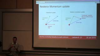
Andrej Karpathy covers the full neural network training pipeline: optimization algorithms like Adam and SGD, batch normalization, dropout regularization, and the history of convolutional networks from Hubel & Wiesel's visual cortex work through AlexNet to modern architectures.
Chapters
OK, so let's dive first. Today we'll talk about training neural networks again, and then I'll give you a bit of an intro to convolutional neural networks. Before we dive into the material, just some administrative things first. First, I didn't get a chance to actually introduce Justin last lecture. Justin is your instructor also for this class, and he was missing for the first 2 weeks. And so you can ask him anything about anything. He's very knowledgeable. Maybe that's an overstatement, but I don't know. [Speaker:ANDREJ KARPATHY] You can try. [Speaker:ANDREJ KARPATHY] OK. And the assignment 2 is out, as a reminder. It's quite long, so I encourage you to start earlier. And it's due basically next Friday. So get started on that as soon as possible. And you'll implement neural networks with the proper API of forward backward passes. And you'll see the abstraction of a computational graph. And you'll implement also batch normalization dropout. And then you'll actually implement convolutional networks. So by the end of this assignment, you'll actually have a fairly good understanding of all the low-level details of how a convolutional neural network classifies images. Okay. So where we are in this class, just as a reminder again, we're training neural networks. And it turns out that training neural networks is really a 4-step process. Um, you have an entire dataset of images and labels. We sample a small batch of that dataset. We forward propagate it through the network to get the loss, which is telling us how well we're currently classifying this batch of data. And then we backpropagate to compute the gradient on all the weights. And this gradient is telling us how we should nudge every single weight in the network so that we're better classifying these images. And then once we have the gradient, we can use it for a parameter update where we actually do that small nudge. We— last class, we looked into activation functions and an entire zoo of activation functions and some pros and cons of using any of these inside your neural network. A good question came up in Piazza. Someone asked, why would you even use an activation function? Why not just skip it? And the question was posted, and I forgot to really address this very nicely in the last lecture. But basically, if you don't use an activation function, then your entire neural network ends up being one single linear sandwich. And so your capacity is equal to that of just a linear classifier. So those activation functions are really critical to have in between. And they, they are the ones that give you all this wiggle that you can use to actually fit your data. We talked briefly about data preprocessing techniques, but very briefly. We also looked at the activation functions and their distributions throughout the neural network. And so the problem here, as you recall, is we have to choose this initial— initialization for our weights. And in particular, there's the scale of how large we want those weights to be in the beginning. And we saw that if that— if those weights are too small, then your activation in a neural network, as you have a deep network, goes all towards zero. And if you set that scale slightly too high, then all of them will explode instead. And so you end up with either supersaturated networks or you end up with networks that just output all zeros. And so that scale is very, very tricky thing to set. We, we looked into the Xavier initialization, which gives you a reasonable kind of thing to use in that form. And that gives you basically roughly good activations or distributions of activations throughout the network in the beginning of training. And then we went into batch normalization, which is this thing that alleviates a lot of these headaches with actually setting that scale properly. And so batch normalization makes this a much more robust choice. So you don't have to precisely get that initial scale correct. And we went into all of its pros and cons, and we talked about that for a while. And then we talked about the learning process. And so I tried to show you kind of tips and tricks for how you actually babysit these neural networks, how you get them to train properly, and also how you run cross-validations and how you slowly converge over time into good hyperparameter ranges. So we talked about all of that last time. So this time we're going to go into some of the remaining items for training neural networks, in particular parameter update schemes, I think, for the most part. And then we'll talk a bit about model ensembles, dropout, and so on. OK? So before I dive into that, any administrative things, by the way, that I'm forgetting? Not necessarily? OK. So parameter updates. So recall that there's this 4-step process to training a neural network. And this is a pseudocode, really, in what it looks like. We get a data batch, evaluate the loss, evaluate the gradient, and perform a parameter update. When I talk about parameter updates, we're specifically looking at this last line in here, where we are trying to make that more complex. So right now what we're doing is called just gradient descent. Where we take that gradient and we— that we've computed, and we just multiply it, scaled by the learning rate, onto our parameter vector. We can be much more elaborate with how we perform that update. And so I flashed this image briefly in the last few lectures, where you can see different parameter update schemes and how quickly they actually optimize this simple loss function here. And so in particular, you can see that SGD, which is what we're using right now in the fourth line here, that's SGD in red, you can see that that's actually the slowest one of all of them. So in practice, you rarely ever use just basic SGD, and there are better schemes that we can use, and we're going to go into those in this lecture. So let's look at what the problem is with SGD. Why is it so slow? So consider this particular slightly contrived example here where we have a loss function surface. So these are the level sets of our loss. And suppose that it's elongated along one direction much more than another direction. So basically, this loss function here is very shallow horizontally, but it's very steep vertically. And we want to, of course, minimize this. And right now we're at the red spot and we're trying to get to the minimum denoted by the smiley face. That's where we're happy. But think about what the trajectory of this is, um, in both x and y directions of SGD if we try to optimize this landscape. What would that look like? So what would it look like horizontally and vertically? I see someone's plot. So what are you plotting out there? [Speaker:AUDIENCE] It's going to bounce more up and down against the horizontal. [Speaker:ANDREJ KARPATHY] OK. And why is it— OK, so why is it going to bounce up and down like that? And why is it not making a lot of progress? [Speaker:AUDIENCE] Because the local gradient is pointing to the— [Speaker:ANDREJ KARPATHY] Right. So the local gradient basically has this form, where when we look at the gradient horizontally, we see that the gradient is very small because this is a shallow function horizontally. But vertically, we have a large gradient because it's a very steep function. And so what's going to happen when you roll out SGD in these kinds of cases and you end up with this kind of pattern where you're going way too slow in horizontal direction, but you're going way too fast in the vertical direction. Okay, so you end up with this ugly jitter. So one way of remedying this kind of situation is what we call a momentum update. So the momentum update will change our update in the following way. So right now we're just incrementing the gradient. We're taking the gradient and we're integrating our current position by that gradient. In a momentum update, instead, we're going to take the gradient that we've computed, and instead of integrating the position directly, we're going to increment this variable v, which I call v for velocity. So we're going to— and we'll see why that is in a bit. So we increment this velocity variable v, and instead, instead, we're basically building up this exponential sum of gradients in the past, and that, that's what's integrating the position. This μ here is a Hoppe parameter. And mu is kind of a number between 0 and 1. And what it's doing is it's decaying the previous v and adding on this current gradient. So what's nice about the momentum update is that you can interpret it in very physical terms and in the following way. Basically, using momentum update corresponds to interpreting this as really a ball rolling around this landscape. And the gradient in this case is your force that the particle is feeling. So this particle is feeling some force due to a gradient. But instead of directly integrating the position, this force— F equals ma in physics, so force is equivalent to acceleration there. And so acceleration is what we're computing. And so the velocity gets integrated by the acceleration here. And then the μ times v has the interpretation of friction in that case, because at every single iteration, we're slightly slowing down. And intuitively, if this μ times v was not there, then this ball would never come to a rest because it would just jiggle around the loss surface forever, and there would be no loss of energy where it would sit settle at the end of a loss function. And so that's the momentum update. It's taking this physical interpretation of optimization where we have a ball rolling around, around, and it's slowing down over time. And so the way this works is— what's very nice about this update is you end up building up this velocity. And in particular, in the shallow directions, it's very easy to see that if you have a shallow but consistent direction, then the momentum update will slowly build up the velocity vector in that direction. You'll end up speeding up and up across the shallow direction. But in a very steep directions, what's going to happen is you start, of course, jittering around. But then you're always being pulled up the other direction towards the center. And with the damping, you end up kind of oscillating to the middle. And so it's kind of damping these oscillations in the steep directions. And it's kind of encouraging these oscillate— it's encouraging process in these consistent shallow directions. And that's why it ends up improving the convergence in many cases. So for example, here in this visualization, we see the SGD update in red. Momentum update is in green. And so you can see what happens with the green one. It overshoots because it's built up all this velocity. So it overshoots the minimum, but then it eventually ends up converging down. And of course, it's overshot, but once it converges there, you can see that it's converging there much quicker than just a basic SGD update. So you end up, uh, building up too much velocity, but then you eventually get there quicker than if you did not have a velocity. Okay? So that's the momentum update. I'll go into a particular variation of the momentum update in a bit. I just wanted to ask, are there any questions about the momentum update at this point? Go ahead. [Speaker:AUDIENCE] Do you typically use one mu for everything, or do you have a different mu for each layer? [Speaker:ANDREJ KARPATHY] Yeah, thank you for asking. So do we use a single mu? And usually we do. That's a single hyperparameter. And usually it takes on values of roughly 0.5 or 0.9. And usually people sometimes— this is not super common, but people sometimes anneal it from 0.5 to 0.99. Slowly over time, but it's just a single number. Go ahead. For this SGD example that you had, couldn't we avoid that problem with a smaller learning rate? Yes. So you could avoid this with a smaller learning rate, but then the issue is, uh, if you had a slower learning rate, this learning rate is applied globally to all the directions in the gradient. And so then you would basically do no progress in the horizontal direction, right? You wouldn't jitter as much, but then it would take you forever to go horizontally if you had a smaller learning rate. So it's this kind of trade-off there. OK? So I'd like to describe a modification on the— oh, sorry. How do we initialize the velocity, or does it matter? Oh, thank you. So v here, the question is, how do you initialize velocity? You usually initialize with 0. And it doesn't matter too much because you end up building it up in the first few steps. And then you end up with this. If you expand out this recurrence, you'll see that basically it's an exponentially decaying sum of your previous gradients. And so once you've built it up, you have a certain amount of it. So initialize at 0. OK? So a particular variation of momentum is called something called Nesterov momentum, or Nesterov accelerated gradient descent. And the idea here is we have the ordinary momentum equation here. And the way to think about it is that your x is incremented by really two parts. There's a part that you've built up some momentum in a particular direction. So that's the momentum step in green. That's the μ times v. That's where your momentum is currently trying to carry you. And then you have the second contribution from the gradient. So the gradient is pulling you this way towards the decrease of a loss function. And the actual step ends up being the vector sum of the two. So the blue is what you end up with, is just the green plus the red. And the idea with Nesterov momentum— and this ends up working better in practice— is the following. We know at this point, regardless of what the current input was to us— so we haven't computed the gradient step yet— but we know that we've built up some momentum and we know we're definitely going to take this green direction. Okay, so we're definitely going to take this green. So instead of evaluating the gradient here at our current spot, Nesterov momentum does this one-step look-ahead and instead evaluates the gradient at this point, this point at the top of the arrow. So what you end up with is the following difference. Here, we know we're going to go this way anyway, so why not just like look ahead a bit to that part of the objective and evaluate the gradient at that point. And at that point, of course, your gradient is going to be slightly different because you're in a different position in loss function. And this one-step lookahead gives you a slightly better direction over there. And you get a slightly different update. Now, you can theoretically show that this actually enjoys better theoretical guarantees on convergence rates. But not only is it true in theory, but also in practice, Nesterov momentum almost always works better than just standard momentum. OK? So the difference roughly is the following. Here I've rewritten it in LaTeX notation instead of code. But we still have this velocity vector equals mu times the previous velocity vector and the gradient that you're currently evaluating. And then we do an update here. And so the Nesterov update, the only difference is we're appending here this mu times v_t minus 1. When we're evaluating the gradient, we have to evaluate it at a slightly different position in this lookahead position. And so that's really a Nesterov momentum. It almost always works better. And now there's a slight technicality here, which I don't think I'm going to go into too much. But it's slightly inconvenient, um, the fact that normally we think about just doing a forward pass and backward pass. So what we end up with is we have a parameter vector theta and the gradient at that point. But here Nesterov wants us to have a gradient parameter theta and a gradient at a different point. So it doesn't quite fit in with, like, a simple API that you normally have in your code. And so it turns out that there's a way, and I don't want to really probably spent too much time on this. But there's a way to basically do a variable transform where you denote this to be phi. You do some rearrangement, and then you get something that looks much more like a vanilla update that you can just swap in for momentum, or you can swap it in for SGD. Because you end up with only needing gradient at phi, and you do updates on phi. And this phi is really the looked-ahead version of the parameters instead of just the raw parameter vector. So that's just a technicality. You can go into notes to check this out. OK, so here, Nesterov accelerated gradient is in magenta. And you can see the original momentum here overshot by quite a lot. But because Nesterov accelerated momentum has this one-step lookahead, you'll see that it curls around much more quickly. And that's because all these tiny contributions of a slightly better gradient at where you're about to be end up adding up, and you almost always converge faster. OK, so that's Nesterov accelerated momentum. So until recently, SGD momentum was the standard default way of training convolutional networks. And many people still train using just momentum update. So this is a common thing to see in practice, and even better if you can use Nesterov accelerated momentum. So NAG here stands for accelerated gradient. OK? Question? So in practice, how close together are the minima typically? As in, what's the serious risk of overshooting against that? You're asking about the optimization landscape, and you're thinking about minima and whether or not you can maybe overshoot to a wrong minimum or something like that. So I think it's slightly incorrect to— so when you think about loss functions for neural networks, usually you think about these crazy ravines and lots of local minima everywhere. That's actually not a correct way to look at it. That's a correct approximation to have conceptually in your mind when you have very small neural networks. And people used to think that local minima are an issue in optimizing neural networks. But actually, it turns out with a lot of recent, even theoretical work, that as you scale up your models, these local minima just become less and less of an issue. So the picture to have in mind is there are lots of local minima, but they're all about the same, actually, loss. That's a better way to look at it. So these functions, neural networks, actually in practice end up looking much more like a bowl instead of a crazy ravine landscape. And you can show that as you scale up the neural network, the difference between the worst and your best local minimum, it actually kind of shrinks down over time with some recent results. So basically, there's no bad local minima. This only happens in very small networks. And in fact, in practice, what you find is if you initialize with different random initialization, you almost always end up getting the same answer, like the same loss in the end. So you don't end up— there's no bad local minima you sometimes converge to, especially when you have bigger networks. Thanks for the question. OK, was there a question over there? So Nesterov has this oscillating feature. How do you— Nesterov has an— oscillating feature? Which part is oscillating? [INAUDIBLE] OK, I think you're jumping ahead maybe by several slides. We're going to go into second-order methods in a bit. OK, so let me jump into another update that is very common to see in practice. It's called AdaGrad, and it was originally developed in the convex optimization literature. And then it was kind of ported over to neural networks, and people sometimes use it. So the AdaGrad update looks as follows. We have this update as we normally see. So this is just basic stochastic gradient descent here, learning rate times your, uh, gradient. But now we're scaling this gradient by this additional variable that we keep accumulating, okay? Note here that this cache which we're building up and is the sum of gradients squared, this cache contains positive numbers only. And note that the cache variable here is a giant vector of the same size as your parameter vector. And so this cache ends up building up the— in every single dimension, we're keeping track of the sum of squares of the gradients, or as we like to sometimes call it, the second moment, although it's the uncentered second moment. And so we keep building up this cache, and then we divide element-wise this step function by the square root of cache. And so what ends up happening here, let's see, so that's the reason that people call it a per- per-parameter adaptive learning rate method because every single, uh, par— every single dimension of your parameter space now has its own kind of like learning rate that is scaled dynamically based on what kinds of gradients you're seeing in terms of their scale. So with this interpretation, what happens with AdaGrad in this particular case if we do this? What happens in the horizontal and vertical direction with this kind of dynamics? [INAUDIBLE] Okay, that's correct. So what you'll see is we have a large gradient vertically, and that large gradient will be added up to cache, and then we end up dividing by larger and larger numbers, so we'll get smaller and smaller updates in the vertical step. So since we're seeing lots of large gradients vertically, this will decay the learning rate. And we'll make smaller and smaller steps in the vertical direction. But in the horizontal direction, it's a very shallow direction, so we end up with smaller numbers in the denominator, and you'll see that relative to the y dimension, we're going to end up making faster progress. So we have this equalizing effect of, um, accounting for this, um, the steepness, and in shallow directions, you can actually, uh, have much larger learning rate than, um, instead of the, the, the vertical directions. And but so that's AdaGrad. One problem with AdaGrad is think about what happens to the step size as we're updating this position. If we want to train an entire deep neural network, this takes for a long time, and we're training this over a long time, what's going to happen in AdaGrad? [Speaker:AUDIENCE] It's going to slow down. [Speaker:ANDREJ KARPATHY] OK, of course. So your cache ends up building up all the time. You add all these positive numbers, goes into your denominator. Your learning rate just decays towards 0, and you end up stopping learning like completely. And so that's not— so that's okay in convex problems perhaps when you just have a bowl and you just kind of decay down to the optimum and you're done. But in a neural network, the stuff is kind of like shuffling around and it's trying to fit your data, and that's like a better way to think of it. And so this thing needs continuous kind of energy to fit your data, and so you don't want it to just decay to a halt. So there's a very simple change to an AdaGrad that was proposed by Geoff Hinton recently. And the idea here is that instead of keeping it completely just the sum of squares in every single dimension, we make that counter a leaky counter. So instead, we end up with this decay rate hyperparameter, which we set to something like 0.99 usually. And then what you're doing is you're accumulating the sum of squares, but the sum of squares is leaking slowly with this decay rate. OK? So we still maintain this nice equalizing effect of equalizing the step sizes in steep or shallow directions. But we're not going to just converge completely to zero updates. So that's called RMSProp. One nice historical fun fact about RMSProp, by the way, is the way it was introduced was— you'd think that it would be a paper that proposed this method, but in fact, it was a slide in Geoff Hinton's Coursera class just a few years ago. And so Geoff Hinton just was giving this Coursera class, and he flashed this slide of like, oh, this is unpublished, but this usually works well in practice. And do this. And it's basically RMSProp. And so I implemented it. Then I saw better results on my optimization right away. And I thought that was really funny. And so in fact, in my papers— not only my papers, but many other papers— people have cited this slide from Coursera. You just slide Lecture 6, this slide. Just that's RMSProp. Since then, this is actually now an actual paper. And there's more results on exactly what it's doing and so on. But for a while, this was really funny. And so in this optimization perspective, we can see AdaGrad here is blue, and RMSProp is this in black. And we can see that both of them converge quite quickly down here this way. In this particular case, AdaGrad ends up converging slightly faster than RMSProp. But that's not always the case. Some— usually what you see in practice when you train deep neural networks is AdaGrad stops too early, and RMSProp will end up usually winning out. In these methods. Any questions about AdaGrad or MSProp? Go ahead. Since you scale down the learning rate in the steeper direction, if the— like in that image that you have— Oh, sorry. Red dot. Where's this image? Yeah. If it was moved over where it was like directly under the smiley face, like don't you want it to just go quickly down the steepest direction? So you're saying that in some cases you might want to actually make faster progress in a steeper direction? The issue is, in this particular case, maybe that's true. But in general, if there are very steep directions, you probably don't want to— this method is saying, don't make very fast updates in that direction. Slow yourself down. So maybe in this particular case, you'd like to go faster, but you're kind of reading into this particular example. And that's not true kind of in general in these optimization landscapes that neural networks are made up of. So this ends up being a good strategy kind of to apply in those cases. Go ahead. So in this, uh, AdaGrad setup, RMSProp, why do we still need the learning rate? Because we have a scaling parameter on the weights anyways, right? [Speaker:ANDREJ KARPATHY] Yeah, but so in the beginning— oh, by the way, I skipped over this explanation of 1e����. But you guys can hopefully see that 1e���� is there just to prevent a division by 0. It's a smoothing factor. It's a hyperparameter. Usually we set it to 1e���� or 6 or 7 or something like that. In the beginning, your cache is 0. So then you increment your— Like, you still need the learning rate to— what you get is this adaptive behavior, but the scale of it is still in your control. The absolute scale of it is still in your control. You still need a learning rate for this. Go ahead. [Speaker:AUDIENCE] Why do we track the past steps? [Speaker:ANDREJ KARPATHY] Like, what it's doing— oh, sorry, just to interrupt. It's kind of doing— you can look at more like a relative thing with respect to different parameters, how are you equalizing the steps. But the absolute global step is still up to you. Go ahead. Why do we track the cache from the very beginning instead of, for example, just the last 100? Why do we cache from the very beginning instead of the last 100? Thank you. So RMSProp is effectively doing what you're describing, right? Because it ends up forgetting gradients from a very long time ago. And its expression at time t is only a function of the last few gradients, but in an exponentially decaying weighted sum. OK, cool. So that's RMSProp. We're going to go into last update. Go ahead. People tried using like a window, like the last, let's say, 10 x squared values that are summed together. So you want to have a finite window over which you're summing up these gradients? Yeah. So would it be similar to RMSProp except— RMSProp is already adding up your gradients from the past in an exponentially weighted way. And so you want to have a finite window on this, or I don't think people have really tried. You can. It takes too much memory. That's what I was thinking. Yeah, it takes too much memory. Although LDFGS kind of has that flavor, but people don't really use that in practice very much. OK. Yeah, so once you're optimizing neural networks, you'll see that X, for example, has 140 million parameters. So that's taking up quite a lot of memory. And so you don't want to keep track of 10 previous gradients and so on. Okay, so last update we're going to go into— oh, sure. Could you, like, combine AdaGrad with momentum? Could you combine AdaGrad with momentum? Thank you for the question. Yes, you could, and that's this slide. So roughly what's happening is Adam is this last update that was only actually proposed very recently, and it kind of has elements of both. As you'll notice, momentum is kind of keeping track of the first-order moment of your gradient. It's summing up the raw gradients, and it's keeping this exponential sum. And AdaGrad and so on are keeping track of the second moment of the gradient and its exponential sum. And what you end up with is an Adam update, is you end up with the step that's basically— it's kind of like— let's see, yeah. It's kind of like RMSProp with momentum a bit. So you end up with this thing that looks like it's— basically keep track of this velocity in a decaying way, and that's your step. But then you're also scaling it down by this exponentially adding up leaky counter of your squared gradients. And so you end up with both in the same formula. And that's Adam update combining those two. So you're doing both momentum and you're also doing this adaptive scaling. And let's see. So here's the RMSProp. Actually, I should have flashed this earlier. So when you compare this, basically RMSProp in red is the same thing as here. Except we've replaced dx, which there was just a previous— just a gradient currently right now. We're replacing this gradient dx with m, which is this running counter of our dx. So if you imagine, for example, one way to look at it also is you're in a stochastic setting, you're sampling mini-batches, there's going to be lots of randomness in the forward pass, and you get all these noisy gradients. So instead of using any gradient at every single time step, we're actually going to be using this decaying sum of previous gradients, and it kind of stabilizes your gradient direction a bit. And that's the function of the momentum here. And the scaling here is to make sure that the step sizes work out relative to each other in steep and shallow directions. Go ahead. So how do you decide on beta 1 and beta 2? Thank you. Beta 1 and beta 2 are hyperparameters. Beta 1 usually 0.9, beta 2 usually 0.995. Somewhere there. So it's a hyperparameter. You have to cross-validate over it. In my own work, I found that this is relatively robust settings across. I don't actually usually end up cross-validating these. I just set them to fixed values usually. Usually. But you can play with those a bit, and sometimes it can help you a tiny bit. OK? Cool. Go ahead. Can you combine Nesterov momentum with AdaGrad? Thank you. So the question is, can you combine Nesterov momentum with AdaGrad? So here, this is like a vanilla momentum. We saw that Nesterov momentum works better. Can you do that? Yes, you can. I actually just read a paper about this yesterday. And actually, it wasn't a paper. It was a project report from 229. Someone actually did that. I'm not sure if there's a paper about it. But yeah, you can play with that, certainly. That's not being done here. OK. One more thing that I— so I have to make Adam slightly more complex here. As you see, it's incomplete. So let me just put in the full complete version. In Adam, there's one more thing where you might be confused when you see it. There's this thing called bias correction that they insert there. And this bias correction, the reason I'm expanding out the loop is that the bias correction depends on your absolute timestep t. So t is used here. And the reason for that is— what this is doing is kind of like a minor point, and I don't want anyone to be confused about this too much. But basically, it's compensating for the fact that M and V are initialized at 0. So your statistics are kind of incorrect in the beginning. And so what it's doing is really it's scaling up your M and V at the first few iterations so you don't end up with a very kind of biased estimate of the first and the second moment. So don't worry about that. Too much. This is only— this is only changing your update at the very first few time steps as, as the Adam is warming up, and so it's done in the proper way in terms of the statistics of MMV. Okay, I don't want to go too much into that. Okay, so we talked about several different updates, and we saw that all these updates have this learning rate parameter still there. And so I just wanted to briefly talk about the fact that all these still require a learning rate, and we saw what happens with different choices of learning rates for all of these methods. The question I'd like to pose is, which one of these learning rates is best to use? Maybe not a well-formed question. I'm trying to trick you. It's a trick question. So when you're running neural networks, this is a slide about learning rate decay. The trick answer is that none of those are good learning rates to use. What you should do is you should use the high learning rate first, because it optimizes faster than the good learning rate. You see, you make very fast progress, but at some point you're going to be too stochastic and you can't converge into your minima very nicely because you have too much energy in your system and you can't settle down into, like, nice parts of your loss function. And so what you do then is you decay your learning rate, and then you can kind of ride this wagon of decreasing learning rates and do best in all of them. So there are many different ways that people decay the learning rates over time, and you should also decay them in your assignment. Uh, there's step decay, which is kind of like the simplest one perhaps, where after one epoch of training data, epoch is referring to you've seen every single training example one time. So after, say, one epoch, you decay the learning rate to— by a factor of 0.9 or something like that. You can also use exponential decay or 1 over t decay. There's several, several of them. I go into notes, uh, slightly expanding on, uh, some of the theoretical properties that have been proven about these different decays. Unfortunately, not many of them applied because I think they're mostly from convex optimization literature, and we're dealing with very different objectives. But usually in practice, I just use exponential decay or something like that. Was there a question? Go ahead. Yeah, I was going to ask the same question about the convergence algorithms. Could you skip from one to the next by using the mean to accelerate your losses at a certain point and then switch to something that's going to converge faster? I see. So you're asking about not committing to any one of these, but you want to also shift between them. During training. Yeah, I don't think that's standard at all. That's an interesting point. I'm not sure when you'd want to use— yeah, it's not clear to me. You could try that in your assignment. That's a fun thing to try. In practice, I'd like to make the point that you almost always— I find, at least in practice right now, Adam is usually the nice default choice to go with. So I use Adam for everything now, and it seems to work quite well, better than Momentum or RMSProp. Or AdaGrad or anything like that. Okay, cool. So these are all first-order methods, as we call them, because they only use your gradient information at your loss function. So we've evaluated the gradient, and we basically know the slope in every single direction, and that's the only thing that we use. There's an entire set of second-order methods for optimization that you should be aware of. The second-order optimization methods, I don't want to go into too much detail, but they end up forming a larger approximation to your loss function. So they don't only approximate it with this basically hyperplane of like which way are we sloping, But you also approximate it by this Hessian, which is telling you how your surface is curving. So you don't only need the gradient, you also need the Hessian, and you need to compute that as well. And you may have seen a Newton method, say, for example, in 229. So a Newton method, it's basically giving you an update that once you've formed your bowl-like Hessian approximation to your objective, you can use this update to jump directly to the minimum of that of that approximation, and then you iterate the scheme. So what's nice about second-order methods? Why do people like these or use them, especially the Newton method as presented here? What's nice about this update? Faster convergence. Faster convergence. Less hyperparameters. Thank you. Less hyperparameters. You'll notice no learning rate, no hyperparameter in this update. And that's because if you see your gradient in this loss function, but you also know the curvature in that place. And so if you approximate it with this bowl, you know exactly where to go, to the minimum of your approximation. So there's no need for a learning rate. You can jump directly to that minimum of that approximating bowl. So that's a very nice feature. I think those are the two that I had in mind. You have a faster convergence because you're using second-order information as well. Why is it kind of impractical to use this step update in training neural networks? Good? [Speaker:AUDIENCE] Your Hessian will be gigantic because you have way too many parameters. [Speaker:ANDREJ KARPATHY] Yeah. So the issue, of course, is Hessian. Say you have a 100 million parameter network, your Hessian is 100 million by 100 million matrix, and then you want to invert it. [LAUGHTER] So good luck with that. So this is not going to happen. So there are several kind of algorithms that I'd just like you to be aware of. We're not going to use them in this class. But just be aware that there's something called BFGS, which basically lets you get away with not inverting the Hessian. It builds up an approximation of the Hessian through successive updates that are all rank 1, and it kind of builds up this Hessian. But you still need to store the Hessian in memory, so still no good for large networks. And then there's something called LBFGS, short for Limited Memory BFGS, which does not actually store the full Hessian or its approximated inverse, and that's what people use in practice sometimes. Now, LBFGS, you'll see it sometimes mentioned in optimization literature especially. What it works really, really well for is if you have a single small deterministic function like f(x), there's no stochastic noise— like, there's no stochasticity in f, and everything fits in your memory, then LBF-GS can usually crush these loss functions very easily. But what's tricky is to extend LBF-GS to, uh, basically very, very large datasets. And the reason is that we're subsampling these mini-batches because we can't fit all the training data into memory. So we subsample mini-batches, and then LBF-GS kind of works on these mini-batches, and its approximations end up being incorrect as you swap different mini-batches. Also, the stochasticity, you have to be careful with it, and you have to make sure that you fix dropout. You have to make sure that your function— Internally, LBFJS calls your function many, many different times as it's doing all these approximations and line search and stuff like that. It's a very heavy function, and so you have to make sure that when you use this, you disable all sources of randomness because it's really not going to like it. Basically, in practice, we don't use LBFJS because it seems seems to not work really well right now compared to first-order methods. It's basically too heavy. Too much stuff is happening. And it's better to just do this noisier stuff but do more of it. That's the trade-off. So in summary, use Adam as a good default choice. And if you can afford to— you can afford full batch, so maybe your dataset is not very large and you can afford to have it all in memory and do all the forward and negative passes in memory, then you can look into LBFGS. But you won't see it in practice used in any large-scale setting right now, although it's a research direction right now. All right, so that concludes my discussion of different parameter updates, decay or learning rates. We're not going to look into all BFGs in this class. There's a question in the very back. Yes, we talked about why it's good to decay your learning rates, but also why the adaptation suffers because if you decay your learning rates, —gradient type of update? So I'm not sure if I fully understood your question. You're asking about— so AdaGrad, for example, it automatically decays your learning rate over time. So would you use also learning rate decay if you're using AdaGrad? So usually you see learning rate decay very common when you do SGD or SGD momentum. I actually am not sure if you'd use it with AdaGrad or Adam. I've used your learning rate decay with Adam before. Before. It tends to help a little bit, but it kind of breaks some of the theory. But it does help sometimes. Yeah, it's not— yeah, yeah. So not a very good answer there. You can certainly do it, but maybe Adam is not— like, Adam will not just monotonically make your learning rate 0 at the end, right, because it's a leaky gradient. But if you used AdaGrad, then certainly decaying the learning rate probably does not make sense because it's decayed automatically to 0 in the end. All right, cool. OK, so we're going to go into model ensembles. I'd just very briefly like to talk about it because it's quite simple. Turns out that if you train multiple independent models on your training data instead of just a single one, and then you average their results at test time, you always get 2% extra performance. OK? So this is not really a theoretical result here. It's kind of like an Andrej Karpathy result, but just like in practice, basically, this is like a good thing to do, almost always works better. The downside, of course, is now you have to have all these different independent models, and you need to do forward and back— forward passes of all of them, and you need to have trained all of them. So that's not ideal because you have a linear slowdown test time with the number of models in your ensemble. And so there are some tips and tricks for using ensembles but kind of faking it a bit. So one approach, for example, is as you're training your neural network, you have all these different checkpoints. Usually you're saving them every single epoch. You save a checkpoint and you figure out what your— was your validation performance. So one thing you can do, for example, it turns out to actually give slight boost sometimes, is you just, uh, take, um, some different checkpoints of your model and you do an ensemble over those. That actually turns out to sometimes improve things a bit. And so that way you don't have to train 7 independent models, you just trained one, but you ensemble some different checkpoints. Related to that, uh, there's a trick of, For test— okay, so what's happening here, this is your 4 steps that we've seen before. I'm keeping another set of parameters here, X test, and this X test is a running sum, exponentially decaying, of my actual parameter vector X. And when I use X test in validation or test data, it turns out that this almost always performs slightly better than using X alone. Okay, and so this is kind of doing like a small, like, weighted ensemble of last previous few parameter vectors. It's kind of a It's kind of difficult to interpret actually, but basically one way to interpret it, one way I can handwave about why this is actually a good thing to do is think about optimizing your bowl function and you're stepping too much around your minimum. Then actually taking the average of all those steps gets you closer to the minimum. OK, so that's the handwaving I can do for why this actually ends up working slightly better. So that's model ensembles. I had to discuss model ensembles because we're going to look into dropout. And this is a very important technique that you will be using and implementing and so on. So the idea for dropout is very interesting. What you do with dropout is you— as you're doing a forward pass of your neural network, you will randomly set some neurons to 0 in the forward pass. Okay? So just to clarify, what you will do is as you're doing a forward pass of your data x, you're computing, say, in this function, your first hidden layer is the nonlinearity of w1 times x plus b1. So that's the activations of the first hidden layer. And then I will compute here a mask of binary numbers, either 0 or 1, based on whether or not numbers between 0 and 1 are smaller than p, which we here see is 0.5. So this U1 is a binary mask of 0s and 1s, half and half, and then we multiply that onto our hidden activations, effectively dropping half of them. So we've computed all the activations h1, the hidden layer, and then we drop half the units at random. And then we do second, and then we drop, half of them at random. Okay? And of course, uh, this is only the forward pass. The backward pass has to be appropriately adjusted as well. So these drops have to be also backpropagated through. So remember to do that when you implement dropout. So it's not only in the forward pass you drop, but in the backward pass you have to backpropagate through multiplying by u2 and by u1. So you kill gradients basically in places where you've dropped a unit. Okay. So you might be thinking when I showed you this for the first time, How does this make any sense at all? And how is this a good idea? Why would you want to compute your neurons and then set them at random to 0? How does that make any sense whatsoever? So I don't know. What do you guys think? Go ahead. Would it prevent overfitting? Would it prevent overfitting? In what sense? It could probably give— instead of getting some neurons. I guess it would make it— force it to be more diffuse over time. [Speaker:ANDREJ KARPATHY] OK. You're roughly getting the right intuition. So you're saying it will prevent overfitting because if I'm only using half of my network, then roughly I have smaller capacity. I'm only using half of my network at any one time. And with smaller networks, there's only so much I can do with half a network than as a full network. So it's kind of like a control of your variance. In terms of what you can represent. Go ahead. [Speaker:AUDIENCE] That is the same thing. A variance of the— it sees a lot of different variance in the input. [Speaker:ANDREJ KARPATHY] Yeah. Yeah. OK. I would like to be slightly careful with the terms like bias-variance trade-off and so on. I haven't really— we're not going into that too much. But yeah, basically, a smaller model, it's harder to overfit. Good. [Speaker:AUDIENCE] It's like having many ensembles of neural networks. [Speaker:ANDREJ KARPATHY] OK. You're saying it's like having many ensembles of different neural networks. We're going to go into that point in a bit. Pardon? It's forcing all the neurons, all the individual neurons to be useful and not just allow one particular one to be useful. Because when that gets dropped off, you get a big negative result. OK. So you're saying that it's forcing all the neurons to be useful because if one of them gets dropped out, then if that one was the only one that was used upstairs, Okay, I have a better way of rephrasing that point in my next slide. Let's look at a particular example instead of hand waving, okay? Suppose that we are trying to compute the cat score in the neural network, okay? And the idea here is that you have all these different units, and what dropout is doing is it's forcing— there are many ways to look at dropout, but one of them is it's forcing your code, your representation for what the image was about, to be redundant. Because you need that redundancy because you're about to, in a way that you can't control, get half of your network dropped off. And so you need to base your cat score on many more features if you're going to correctly compute the cat score, because any, any one of them you can't rely on it because it might be dropped. And so that's one way to look at it. So in this case, we can still classify cat score properly even if we don't have access to whether or not it's furry or mischievous and so on. Um, so that's one interpretation of dropout. Okay, another interpretation of dropout is, as was mentioned, in terms of an ensemble. So dropout is effectively— can be looked at as training a large ensemble of models that are basically subnetworks of this one large network, um, but they kind of share parameters in a weird way. So to understand this, you have to notice the following. If we do a forward pass and we randomly drop off some of the units, then in backward pass, think about what happens with the gradient, right? So suppose we've ran— randomly dropped off these units, In a backward pass, we're backpropagating through the masks that were induced by dropout. So in particular, only the neurons that were used in the forward pass will actually be updated or have any gradients flowing through them. Because any neuron that was shut off to 0, no gradient will flow through it, and its weights to its previous layer will not be updated. So effectively, any neuron that was dropped out, its connections to the previous layer will not be updated. And it would just— it's as if it wasn't there. So really with the dropout masks, you're subsampling a part of your neural network, and you're only training that neural network on that single example that you have at that point in time. So each binary mask is one model and gets trained on only one data point. I'm not sure what you said. I can try to repeat that. It came from somewhere here. I'm on to you guys. OK. But do people actually understand this, or nods, or— OK. So when you drop a unit, you drop a neuron. I wish I had the example of the neuron, right? But if I drop its value, I multiply its output by 0. Then its effect on the loss function, there's no effect, right? So its gradient will be 0 because its value was not used in computing the loss. And so its weights will not get an update. And so it's as if we've subsampled a part of the network and we only train that single data point that currently came to the network. We only train on it. And every time we do a forward pass, we subsample a different part of your neural network, but they all share parameters. So it's kind of like a weird ensemble of lots of different models all trained on one data point. But they all share parameters. So that's kind of roughly the idea here. Does that make sense? OK, cool. Go ahead, question? What percentage of the neurons in a network get dropped out? Usually, say, 50% is a very rough approximation you can use. And then do your weight arrays, do they still stay the same size, or are there ways to scale down the weight arrays in a layer? Yeah, the weight array is the same size. In this forward pass, you'll notice we actually compute all the neurons h. We compute them just as we did before. All of the neurons get computed, but then half of the values will get dropped to 0. So nothing changes there. Just scale it— oops, sorry— times 2 or something like that. Oh, yes. So we'll see that in a bit. Go ahead. Wouldn't you be making the matrix sparse so you can use a bunch of sparse matrix optimizations when you do the calculations? Would you be making the matrix sparse so can you take advantage of some sparse matrix computations? So instead of computing all the h's, you want to only compute the neurons that are not being dropped. And in that case, you want to do sparse updates. So you could in theory, but I don't think that's done usually in practice. We don't worry about it too much. So I guess it would depend on what neurons get dropped out, right? So but like iterating over all combinations is a bad runtime. So how do you choose which ones to drop? Oh, I see. So in every single forward pass, we sample these. We sample the mask at every single forward pass. And so you always get a different subnetwork that you're training. So every single iteration, we get a mini-batch. We sample our noise pattern for what we're going to drop out. And we do a forward and backward pass and update the gradient. And we keep iterating this over and over again. But is there a potential algorithm to precisely choose the good— Oh, I see. So your question is, can we somehow cleverly choose the binary mask in a way that best optimizes the model or something like that? Not really. I don't think that's done or anyone has looked into it too much. Go ahead. [INAUDIBLE] Sorry? Do we do the dropout for test purposes? Oh, yes. So I'm going to get into that in one slide. In the next slide, we're going to look at test time. I'll take one last question. Go ahead. Have you applied different masks? [INAUDIBLE] [Speaker:ANDREJ KARPATHY] So two questions. One is, can you use dropout to different amounts in different layers? You can. There's nothing stopping you. Intuitively, you want to apply stronger dropout if you need more regularization. So if there's a layer that has a huge amount of parameters— we'll see that in ConvNets in one example— you want to apply stronger dropout there. Conversely, there might be some layers that we'll see with convolutional networks early on the convolutional layers are very small. You don't usually apply as much dropout there. So it's quite common, for example, in the convolutional network— and I'll go into this in a bit— you start off with low dropout and then you scale that up over time. So the answer to that is yes. And I forgot your second question. What was it? Uh, dropout on weights. Oh, can you instead of units dropout just individual weights? You can, and that's called something called DropConnect. We won't go into it too much in this class. But there's a way to do that as well. Okay. Now at test time, at test time ideally what you want to do is we've introduced all this noise, right, into the forward pass. And so what you— what we'd like to do now at test time is we'd like to integrate out all that noise. And a Monte Carlo approximation to that would be something like you have a test image that you'd like to classify. You can do many forward passes with many different settings of your binary masks, and you're only using the subnetworks. And then you can average across all those probability distributions. So that would be great, but unfortunately it's not very efficient. So it turns out that you can actually approximate this process to some degree, as Geoff Hinton pointed out when he first introduced dropout. And the way we'll do this— intuitively, you want to take advantage of all your neurons. You don't want to be dropping them out at random. So we're going to try to come up with a way where we can leave all the neurons turned on, so do no dropout in a forward pass on a test image. But we have to actually be careful with how we do this. Um, so we can— so in a forward pass for test images, we're not going to drop any units, but we have to be careful with something. Uh, and, uh, basically one way to get at what the issue is, is suppose that this was a neuron and it's got two inputs. And suppose that it, uh, with all these inputs present at test time, so we're not dropping units. So we're at test time, these two have some activations, and the output of this neuron gets computed to be some value x. You have to compare this value of x to what the neuron's output would be during training time in expectation. Okay, because in, in training time, this dropout masks very randomly, and so there's many different cases that could have happened. And in different— in those cases, the outputs of this neuron would be possibly in a different scale, and you have to worry about this. So let me show you exactly what this means, I think. So during test, this neuron computes— say there's no nonlinearity, we're only looking at a linear neuron. During test, test, this activation becomes w0, which is the weight here, times x plus w1 times y. Okay? So that's what we want to compute at test time. And the reason we have to be careful is that during training time, the expected output of a in this particular case would have been quite different. So we have 4 possibilities. We could have dropped one or the other or both or none. So in those 4 possibilities, we would have computed different values. And if you actually crunch through this math, you'll see that when you reduce it, you end up with 1/2 of w_0x plus w_1 times y. So in expectation at training time, the output of this neuron was actually a half of what it is at test time. Okay? And so when you want to use all the neurons at test time, you have to compensate for this additional half. And that half, by the way, is coming from the fact that we've dropped units with probability of a half. And so that's why this ends up being a half. And so with probability 0.5, uh, all inputs in a forward pass, uh, so basically if we did not do this, then we end up having too large of an output compared to what we had in expectation during training time. And your output distribution would change. And basically things in the neural network would break because they're not used to seeing such large outputs from all the neurons. And so you have to compensate for that and you have to, squish down. So now you're using all your things instead of just half of the things, but you have to squish down the activations to get back the— to recover your expected output. Okay, this is actually a tricky point. By the way, I think I was told once a story that when Geoff Hinton came up with dropout, in the beginning he actually didn't fully come up with this part. So he tried dropout and it didn't work. And actually the reason it didn't work is he, um, he missed out on this tricky point actually, admittedly. And so you have to scale your activations at test time down because of this effect. And then everything works much better. So at test time, just to show you what this looks like, we basically compute these neural nets as normal. So we compute the first hidden layer, second hidden layer. But now at test time, we have to multiply by p. So for example, if p is 1/2, we're dropping out with a half probability. Then we're scaling down the activation so that the expectation the expected output now is the same as expected output in the training time. And so at this time, you actually recover full dropout and, uh, and the expected outputs are matching and this actually works really well. Go ahead. At training time, one quarter of the time I will actually have the same problem, right? Because both neurons will be active. And so I assume due to the scaling, is that a problem for training? Does it slow down training? So, um, in training we're half the time dropping these inputs and so you end up with some, some expected output from this neuron. I don't think there's an issue at train time, basically. It's just the discrepancy between train and test. Like, if you're using all your neurons instead of dropping them, there's discrepancy. So either you can correct it at test time, or you can use what we call inverted dropout, which I'll show you in a bit. So let me just get to that in a bit. So dropout summary: if you want to use dropout, drop your units with probability of— with keeping a probability of p, and then at test time, don't forget to scale them. So if you do this, your neural networks will do— will work better. Okay? And don't forget to also backpropagate the masks, which I'm not showing here. An inverted dropout, by the way, to, um, is to take care of this discrepancy between the train and test distribution in a slightly different way. In particular, what we'll do is we're changing this step here. So before, U1 was a binary mask of 0s and 1s. What we're now going to do is we're going to do the scaling here at training time. So we're going to scale down the activations at training time, or rather scale them up, because if p is 0.5, then we're boosting activations at training time by half. And then at test time, we can leave our code untouched. So we're doing the boosting of the activations at training time. We're making everything artificially greater by 2x. And then at test time, we're supposed to half, but now we're just going to recover the clean expressions because we've done the scaling at training time. So now you'll be properly calibrated in expectations between the train and test. Of every neuron in the network. OK? So that's dropout. So use inverted dropout. That's the most common one to use in practice. So in effect, it really comes down to a few lines. And then the backward pass changes a bit. But the networks almost always work better with this. Go ahead. Unless you're severely underfitting. Go ahead. When you sort of make the approximation that the neurons are you're going to see the expected value of like the weights after dropout. Does that depend on you having a linear response in activation function? Thank you for the question. Does that depend on you having a linear response activation function? It does. So once you have nonlinearities in there, then these expectations aren't actually exact. And that's why this is an, as I mentioned here, approximation. It's an approximation to evaluating the full ensemble. And one of the reasons it's an approximation is because once you actually have nonlinearities in the picture, then these expected outputs are all kind of screwed up because of the nonlinear effects on top of these. So yeah, that's a good question. Thank you for pointing that out. Go ahead. Since it's nonlinear, you— like, inverted dropout and dropout are not equivalent in terms of the final model. I see. You're saying that the inverted dropout and dropout are not equivalent. So doing inverted dropout or not is not equivalent because of the nonlinearities? I'd have to think about it. Maybe you're right. Yeah, maybe you're right. Yeah. Yeah. Go ahead. So in the inverted dropout, why do you think dividing by p rather than— you can imagine instead dividing by the mean of the mask. So p here is 0.5, right? So with probability of 0.5, we're dropping. Selected either— like, the number you selected is binomial, right? So you may have selected a really small network or a really big network. And you can imagine— I see. So sometimes you have more dropped and less dropped. Then you have an entire distribution. Like, in some forward passes, you'll have fewer neurons than half or more neurons than half. But I think all of this is just about expectations. In expectation, you're dropping half. And so that's the correct thing to use, even though there's some randomness on exactly the amount that actually end up being dropped. OK, great. Oh yeah, this is a placeholder slide to tell you guys a fun story about dropout. So I was in a deep learning summer school in 2012. And Geoff Hinton was for the first time, or at least the first time I saw it, presenting dropout. And so he's basically just saying, OK, set your neurons to 0 at random. And at test time, just boost the activations. And this always works better, better. And we're like, wow, that's interesting. And so a friend of mine sitting next to me, he just pulled up his laptop right there. He has a station of his university machines. And he implemented it right there during the talk. And by the time Geoff Hinton finished the talk, he was getting better results and getting actually state-of-the-art report— like, accuracies on his dataset that he was working with. So that's the fastest I've seen someone go, like, get an extra few boost percent. It was right there and then while Geoff Hinton was giving the talk. So I thought that was really funny. There's very few times that actually something like this happens. And so dropout is a great thing because it's one of those few advances that is very simple and it always works, just better. And there's very few of those kinds of tips and tricks that we've picked up. And I guess the question is, how many more simple things like dropout are there that just give you 2% boost always? So we don't know. OK. So I was going to go at this point into gradient checking. But I think— actually, I decided that I'm going to skip this because I'm tired of all the neural network— like, we've been talking about lots of details of training neural networks, and I think you guys are tired as well. And so I'm going to skip gradient checking because it's quite well described here in notes. So I encourage you to go through it. Gradient checking is kind of a tricky process. It takes a bit of time to appreciate all the difficulties with the process. And so just read through it. I don't think there's anything I can hand wave around to make it more interesting to you. And so I would encourage you to just check it out. Meanwhile, we're going to jump right ahead and go into convolutional networks and look at pictures. Convolutional neural networks look like this. This is a LeNet-5 from 1980, roughly. And so we're going to go into details of how convolutional neural networks work. And in this class, we're not actually going to do any of the low-level details. I'm just going to try to give you intuition about how this field came about, some of the historical context, and just kind convolutional networks in general. So if you'd like to talk about the history of convolutional networks, you have to go back to roughly 1960s to experiments of Hubel and Wiesel. So in particular, they were studying the prime— the visual cortex in a cat. And they were studying an early visual area in the cat brain as the cat was looking at patterns on the screen. And they ended up actually winning a Nobel Prize for this sometime later for these experiments. And so I'd like to show you what these experiments look like, just so— they're really fun to look at. So I pulled up a YouTube video here. And so what's going on here is the cat is fixed in position, and we're recording from its cortex somewhere in the first visual area of processing, which is in the back of your brain called V1. And now we're showing different light patterns to the cat, and we're recording and hearing the neurons fire for different stimuli. So let's look at how this experiment looked like. I don't know if you guys can hear. So nothing happens when it goes this way, and then he's going to make it go that way. Okay, I don't know if you guys can hear it all the way in the back. Okay, so this is one neuron in the V1 cortex, and through experiments like this, they basically figured out that there are these cells, and they seem to turn on for edges in a particular orientation, and they get excited about edges in one orientation. Any other orientation does not excite them. Okay, and so like this, through a long process, this is like a 10-minute video, so We're not going to go through it. But basically, for a long time, they experimented, and they came up with a model of how the visual cortex processes information in the brain. And so they found several things that ended up leading to their Nobel Prize. For example, they figured out that the cortex is arranged retinotopically, the visual cortex. And what that means is that— let's see, where's my pointer— basically, nearby cells in the cortex— so this is cortical tissue unfolded. Nearby cells in your cortex are actually processing nearby areas in your visual field. So your— whatever is mapping onto your retina is processed nearby in your brain. This locality is preserved in your processing. And they also figured out that there was an entire hierarchy of these— what's called the simple cells, and they responded to a particular orientation of an edge. And then there were all these other cells that had more complex responses. So for example, some cells would be turning off for a specific orientation, but were slightly translationally invariant. So they didn't care about the specific position of the edge, but they only cared about the orientation. And so they hypothesized through all of these experiments that the visual cortex has this kind of hierarchical organization where you end up with simple cells that are feeding to other cells called complex cells, and et cetera. And these cells are building on top of each other. And these simple cells in particular have these relatively local receptive fields, and then we're building up more and more complex representations in the brain through successive layers of representation. And so these were experiments by Hubel and Wiesel, and of course they— some people are trying to reproduce this in computers and trying to model the visual cortex with code. And so one of the first examples of this was the Neurocognitron from Fukushima, and he basically ended up setting up a layered architecture with these local receptive cells that basically these are neurons that look at a small region of the input, and then he stacked up layers and layers of these. And, uh, so he had these simple cells and then complex cells, simple cells, complex cells, and a sandwich of simple and complex cells building up into a hierarchy. Now, back then though, in the 1980s, backpropagation was still not really around, and so Fukushima had an unsupervised learning procedure for training these networks with, like, a clustering scheme, but this was not backpropagated through at the time, but it had this idea of successive layers, small cells building up on top of each other. And then Yann LeCun took these experiments further, and he kind of built on top of Fukushima's work, and he kept the rough architecture and layout, but what he did was actually train these networks with backpropagation. And so, for example, he trained different classifiers for digits or letters and so on, and so trained all of it with backprop. And they actually ended up using this in complex systems, that read check— they read off like digits from postal mail service and so on. And so ConvNets actually go back to quite a long time ago, to 1990s and so on, when Yann LeCun was using them back then. But they were quite small, okay? And so in 2012 is when the ConvNet started to get quite a bit bigger. So this was the paper from— that I keep referring to from Alex Kruchevsky, Ilya Sotskever, and Geoff Hinton. And they took all of ImageNet. ImageNet is a dataset that comes actually from Fei-Fei's lab, from our lab. So it's a million images with 1,000 classes, huge amount of data. You take this model, which is roughly 60 million parameters, and it's called an AlexNet based on the first name of Alex Krizhevsky. These networks we're going to see that they have names. So this is AlexNet. There's a VGGNet, a ZFNet, GoogleNet. There's several nets. So just like this one is LinNet. And so we give them names. So this was AlexNet, and it was the one that actually outperformed by quite a bit all the other algorithms. What's interesting to note historically is the difference between AlexNet in 2012 and the LinNet in 1990s. There's basically very, very little differences when you look at these two different— these two networks. This one used, I think, sigmoids or tanh, tanh probably, and this one used ReLU. And it was bigger and deeper, and it was trained on GPU, and it had more data. and that's basically it. That's the only— like, that's roughly the difference. And so really what we've done is we figured out better ways of, of course, initializing them, and it works better with BatchNorm, and ReLUs work much better. But other than that, it was just scaling up both the data and the compute. But for the most part, the architecture was quite similar. And we've done a few more tricks. Like, for example, they used big filters. We'll see that we use much smaller filters. We also now— this is only a few tens of layers. We now have 150-layer ConvNets, so we've really just, uh, scaled this up quite a bit in some respects. But otherwise, the basic concept of how you process information is similar. Okay? So ConvNets are now basically everywhere. Uh, so they can do all kinds of things like, um, classify things, of course. They're very good at retrieval. So if you show them an image, they can retrieve other images like it. Um, [CLEARS THROAT] they can also do detection. So here they're detecting dogs or horses or people and so on. You'll— this might be used, for example, in self-driving cars. I'll have this on the next slide. They can also do semantic segmentation, so every single pixel is labeled, for example, as a person or a road or a tree or sky or building. So that's segmentation. So they're used in cars. For example, here's an NVIDIA Tegra, which is a small embedded GPU. We can run ConvNets on these, and for example, this might be useful in a self-driving car where you can identify identify all the— you can basically do perception of around you, of things around you. ConvNets are identifying faces. Probably if some of your friends are tagged on Facebook automatically, it's almost certainly, I would guess at this point, ConvNet. They're used on video classification on YouTube, identifying what's inside YouTube videos. They're used in— this is a project from Google that was very successful where basically Google was really interested in taking Street View images and automatically reading out house numbers from them. Okay, and turns out this is a perfect task for a ConvNet. So they had lots of human laborers annotate huge amounts of this data and then put a giant ConvNet on it, and it ended up working almost as well as a human. And that's a theme that we'll see throughout, that this stuff works really, really well. They can estimate poses. They can play computer games. They detect all kinds of cancer or something like that in bio— bio— bioimages. They can read Chinese characters, recognize street signs. This is, I think, segmentation of neural tissue. They can also do things that are not visual. So for example, they can recognize speech. So ConvNets have been used for speech processing. They've been used also for text documents. So you can feed text into ConvNets as well. They've been used for— to recognize different types of galaxies. They've been used to— in the recent Kaggle competition to recognize different whales. So this is a particular whale. There was like 100 whales or something like that, and you have to just use a ConvNet to recognize specific individual whales. So this whale, by the pattern of its, you know, white spots on its head, is a particular whale that the ConvNet has to recognize. So it's amazing that that works at all. They're used on satellite images quite a bit because now there are several companies that have lots of satellite data, so this is all analyzed with large ConvNets. In this case, it's finding roads, but you can also look at agriculture applications and so on. They can also do image captioning. So you might have seen some of these results, my work included as well, where you take images and you caption them with sentences instead of just a single category. And they can also be used for various artistic endeavors. So this is something called DeepDream. And we're going to go into how this works. You'll actually implement it, I think, on your third assignment, maybe? Hopefully. OK. Maybe you will implement this on your third assignment. You give it an image and use using ConvNet, you can make it do weird stuff. In particular, you'll notice there are lots of hallucinations of dogs. And we're going to go into why dogs appear. It has to do with the fact that ImageNet, which is where these networks get trained, they end up— they have a lot of dogs. And so these networks end up hallucinating dogs. It's kind of like they're used to some patterns. And then when you show them a different image, you can make them— put them in a loop with the image and they'll hallucinate hallucinate things. So we'll see how this works in a bit. I'm not going to explain the slide, but it looks cool. So you can imagine that a ConvNet is probably involved somewhere. I also wanted to point out that what's interesting, there's this paper called Deep Neural Networks: Rival Representation of Primate IT Cortex for Core Visual Recognition. What they did here is they are basically looking at— I think this was a macaque monkey. and they're recording from the IT, from the IT cortex here, and they're recording the neural activations as a monkey is looking at images, and then they fed the same images to a convolutional neural network, and what they're trying to do is from the convolutional neural network code or from the population of neurons that is only a sparse population of neurons in the IT cortex, they're trying to perform a classification of some concepts, and what you see is that decoding from the IT cortex and classifying images is almost as good as using this neural network from 2013. So in terms of the information that's there about the image, you can do almost equal, uh, in performance for classification. Um, perhaps even more striking results here where they were comparing— they fed a lot of images through the convolutional network and they got this monkey to look at lots of images. And then you look at how these images are represented in the brain or in the ConvNet. So these are two spaces of representation of how images are arranged in the space by the ConvNet. And you can compare the similarity matrices and statistics, and you'll see that the IT cortex and the ConvNets are basically very, very similar representation. There's a mapping between them. It almost seems like similar things are being computed. The way they arrange the visual space of different concepts and what's close and what's far is very, very remarkably similar to what you see in the, in the brain. And so some people think that this is just some evidence that ConvNets are doing something something brain-like, and that is very interesting. So the only question that remains then in that case is, how do ConvNets work? And we'll find out in the next class. So that's it. OK.
More from Andrej

Skill Issue: Andrej Karpathy on Code Agents, AutoResearch, and the Loopy Era of AI







Andrej Karpathy: Tesla AI, Self-Driving, Optimus, Aliens, and AGI | Lex Fridman Podcast #333