CS231n Winter 2016: Lecture 7: Convolutional Neural Networks

Andrej Karpathy explains how convolutional neural networks work, from filters and pooling through historic architectures like AlexNet and ResNet. He walks through the four key hyperparameters of a convolutional layer and shows how learned filters detect edges, then traces the trend from large filters to many small ones across LeNet, VGGNet, GoogleNet, and ResNet.
Chapters
So today we finally get to cover convolutional neural networks. So we're super excited. But first, let me dive into some administrative items. As a reminder, again, assignment 2 is due next Friday. How's assignment 2 going, by the way? Did people finish the fully connected stuff at all? Some people? OK. How about— did anyone finish batch norm? OK. OK. All right. Thing to worry about perhaps for you guys is the project proposal, which is due very soon on Saturday. It's ungraded. We just want a paragraph. We want to make sure that you guys are on the right track, you've thought about the project, you have a rough proposal for what you want to do. You can also send us a few possibilities, like— and by few I mean two. Don't send us like hundreds. But— and we can help you choose a bit. But yeah, so project proposal due soon. OK, so we are working with neural networks. We're training neural networks in a 4-step process. Last, um, class, we talked about parameter updates. So we covered a whole bunch of parameter updates. Uh, we covered Adam, which is not on that image, and we did not cover AdaDelta, which is on that image. But AdaDelta is kind of analogous to the other parameter updates that I've covered last time. We also talked about dropout, and I introduced briefly convolutional neural networks, and I talked about some of the history of the field and how this developed. So I talk particularly about the experiments of Hubel and Wiesel in the 1960s with the cat visual cortex and their takeaways from a lot of this research, which is that the hierarchical cortex is arranged hierarchically with these simple to complex cells and more and more complex things happening over time. And so today we'll get to dive into some of these models in details, and we'll talk about convolutional neural networks. So first, as I did with neural networks, I'd like to talk about ConvNets without all the brain stuff. So no analogies to neurons or anything like that. We'll just see what the optimal operations are mathematically, and then we'll go into how you can interpret them in terms of neurons being connected in some kind of a simulated brain tissue or something like that. So we start off with some, uh, image. Say this is 32 by 32 by 3 CIFAR-10 image. And as you'll see, convolutional neural networks operate over volumes. All of these layers in between are going to take volumes of activations, and they're going to produce volumes of activations. So our intermediates will not just be vectors like they are with neural networks, but they'll actually have these spatial dimensions of width, height, and depth that will maintain throughout the computation. Now, depth here is not to be confused with a depth of a network. This is just depth as a third dimension of an— of a volume. So in this case, there are 3 channels. So I'll say that this volume of activations is 3 deep. But don't get confused with, like, the depth of a network and the depth of a volume. And so the convolutional layer is the core building block of a convolutional network. And the way convolutional layer works is as follows. We receive some input volume that goes into the layer. And then we'll have all these little filters in a convolutional network. So suppose for now we just have a single filter, and these filters will be small spatially. So spatially, this filter will be only 5 by 5, but it spans— but it will have 3 depth. And so this 3 is always goes through the full input volume. So because the input volume has 3 channels, this filter will be small spatially, 5 by 5, but it will cover the full depth of the input volume, which in this case is 3. And this filter, what we'll do now is we'll take this filter and we'll convolve it over this input volume. And what I mean when I say convolve is we're going to slide it spatially through all spatial locations of this input volume, and we're going to be computing dot products along the way. So this filter here, we're eventually going to learn this. This is now our W, and we're going to learn these filters. But just think about this filter as your W's, and you're sliding them through spatially this input volume, and along the way, as we're sliding this filter through, we're computing a W transpose, uh, times x plus b. And the x here is a small piece of your input volume. So it's a small piece of 5 by 5 by 3. Okay? So really what's happening here is that every single position, uh, say in this particular position in the input volume, we're really computing 5 times 5 times 3, which is 75-dimensional dot product, right? And then plus 1 for bias. So 75-dimensional dot products as we're sliding the filter through. Now when you slide this filter through this volume spatially, you'll end up carving out an entire what we call activation map of activations of the responses of that filter at every single spatial position. So sliding this 5x5 filter through the 32x32 input volume will give us a 28x28 activation map of how much this filter likes any spatial position in this input volume. Where the 28 comes from, by the way, is, uh, the following. You'd have to calculate out, and we'll go into much more details of this, but the input is 32 by 32, and we're sliding a 5 by 5 filter through. And it turns out that basically there are 28 unique positions in both width and height that we can put the filter in. So when you slide this filter through one at a time, you end up covering 28 distinct locations. So that's why we have a 28 by 28 activation map that we're producing. And that is the activation of this filter at every spatial location in the input volume. So now what we're going to do is we won't just have a single filter, but we'll actually have an entire filter bank. So suppose that we have a second filter, a green filter, in this convolutional layer, and this filter will also have the same dimensions, 5 by 5 by 3, and we're going to be sliding it through the volume as well, giving rise to a second activation map. And so this activation map is computed independently from the first. These are all independent filters. So what we'll end up with now is we'll have an entire set of filters. So suppose, for example, that this convolutional layer will have 6 filters, and that's just a hyperparameter. So suppose we had 6 of them, then what we'll do is we'll slide every one of them independently through the input volume, computing dot products along the way. And that's actually called the convolutional— convolution operation. Um, and that gives us the— this entire 28 by 28 by 6, um, set of activation maps that are stacked together along the depth dimension. And so what this convolutional layer has done is it has looked at this image and it has re-represented this image, the 32 by 32 by 3, in terms of the activations on this image of those filters. So we end up with a re-representation of the image of size 28 by 28 by 6. And this will be the next input volume that's going to feed in late into later processing. So just to give you a preview of how this will work in the convolutional network, and there's a lot of details to be worked out, but just to give you a hint of what's coming. We're going to have these convolutional layers. They are going to have some number of filters, and these filters will have some spatial extent, like say 5 by 5. And so this conv layer, uh, short for convolution, will be sliding it through. We get, uh, say a 28 by 28 by 6 volume instead of the original volume. And then this will feed into the next convolutional layer. And of course in the middle of always we're going to be applying, uh, activation functions as we did before with neural networks. So we perform convolutions which are these linear operations, then we threshold all the activations at 0. and then we proceed again with another set of convolutional, another convolutional layer with its own filters, maybe of different size. And so in this case, for example, we also have 5x5 filters, and we're going to slide them through this volume now, giving us a rise of 24x24x10, because now suppose we have 10 filters in this second layer. One thing to notice here is that in this second layer, the green layer, the outputs produced in in green here, these filters must have been 5 by 5 by 6 now because 6 is the depth of the input volume. Okay? So those filters are always small spatially, like we'll see 2 or 3, um, they'll be usually like a 3 by 3 or 5 by 5 or something like that. But during— but they always match the input depth of the input volume. So 6 in the second case and 3 in the first case. Okay? And so where this is going is that these— all these filters are initialized randomly, of course, and— but those will become our parameters in the convolutional network. And so what's going to happen intuitively is we'll end up building an entire feature hierarchy. So suppose we have a convolutional network here. This is taken from slides from Yann LeCun. So we'll have all these convolutional layers along the way. And what you'll find is that when you visualize the— this is already a trained convolutional network. When you look at the filters on the very first layer, so say these are little 5 by 5 by 3 filters, you'll find that they will, through backpropagation, tune themselves to become all these little blobs of edge pieces and little color pieces and blobs. And so these are basically the filters in the first convolutional layer when you visualize them. So all of these filters will be looking for these things in the original image when we convolve through. And as you go into deeper and conv— deeper and deeper convolutional layers and we're performing this successive operations of conv and conv on top of each other, you'll end up eventually with the second convolutional layer, for example, it's going to be dot prod— doing dot products over the outputs of the first conv. Layer. And so it's going to be basically putting together all of these little edge pieces and making larger and larger, uh, kind of, um, pieces out of it that these filters here are going to get excited about. So in the second convolutional layer, maybe you'll get a neuron that gets excited about, uh, or a filter that gets excited about like little circles in the image and so on. Because they'll be putting together, um, all of these guys through this— these dot products. And so on until we end up with all of these, uh, we're— we'll end up basically building up all of these templates for all these different object pieces, like little honeycombs, some kinds of things, or circles and so on, extended parts of objects. And so all of this will— is initially all random, and this will all just come about. One point to make here, by the way, is that in this very first convolutional layer, I'm visualizing the raw weights, the 5x5x3 array, but these are not the raw weights, right? This is just a visualization of what these layers are responding to in the original image, right? Because these filters here are still 5x5 spatially, not— this looks larger, but they are operating over and the outputs of these filters, right? So that's just a subtle point I wanted to bring up. And so you end up with an image that's very similar to maybe what Hubel and Wiesel may have imagined, where you have these simple cells looking for, say, for example, a bar of a specific orientation somewhere specifically in the image, okay? And then we're building up the hierarchy of these features and composing them together spatially to get more and more complex responses of different kinds of objects and so on. And so to put this another way, Uh, let's for example consider, uh, this example where we have this input image here, which is a small piece of a car, I believe. And so in this example, we have on the first convolutional layer trained a whole bunch of filters. There are 32 filters of 5 by 5 spatially. And these are example activation maps that what these look like in practice. So say taking this filter here and convolving it spatially over this image gives us an activation map. And, and these activation maps, white corresponds to high, uh, high activations and black corresponds to low activations, low numbers. And so for example, here we have a filter that has a bit of orange stuff in it. And so when you slide this filter through this image, you'll see a lot of activations in this area where there's the headlamp or something like that because there's orange stuff there. So this filter gets happy about that part. And so these are the activation maps produced by these filters. We'll stack them up along the depth and then we'll feed that into the next convolutional layer, which will be putting together combinations of these guys. Over and over again. And so convolutional network will basically have a layout like this, and we'll see how we'll be arranging, uh, all of this soon. But there will be basically 3 core building blocks: a convolutional, uh, layer, uh, rectifier, uh, layer, which is like a nonlinearity, just thresholding. There will be pooling operations, which we'll go into in a bit, and there is a fully connected layer at the very end, uh, which we'll also go into in a bit. But basically the image feeds into in here, and what I'm visualizing here is that every column here is an— is a volume of representation along the way through the convolutional network, and every row here is an activation map. So there are 10 filters, I believe, in the first conv layer, and these are their activation maps. We then have thresholded them, then we did another convolution, and then we thresholded that. We'll do a pooling operation as we'll see, and piece by piece we're basically creating these 3D volumes of higher and higher level kind of abstraction until at the end we end up with some volume. And then these class scores for different classes of CIFAR-10, say, example, will just be a large, um, fully connected layer, meaning that it's just like in a neural network where you have these neurons that look at all— they have connections to everything in the previous volume. So this last volume here will be stretched out into a giant column, and then we'll do a last matrix multiply to get the scores, uh, for all the different classes. So that's what, uh, convolutional layers will be doing. Now, to take a closer look at us, we're going to take a closer look at the spatial dimension of exactly how this 28 came about and what's happening there. But before I dive into some of those details of the spacings here and the sizes of filters and all this mathematics, is there any questions about just the basic organizational kind of layout and what convolutional layers are doing? Go ahead. [Speaker] How do you How do we choose the number of filters? That's a great question for a few slides. So we're gonna go into that. But the basic, um, I'm trying to see if the basic operation makes sense. Go ahead. You can represent the convolution operation as an affine layer, right? So why do we— I mean, if we just train a basic affine layer, it should probably— so does it like just reduce the parameters and train— make the training faster? Uh, yeah. Thank you. So you're saying that we're basically computing dot products and we can represent those as, uh, as an affine layer. So we could have an affine layer that— yes, so I think we'll go into that in a bit. Basically think about it, it's a local connectivity to the input. We're still doing dot products, but not with the full image. And so yes, it's mostly a computational kind of control. Also, as we'll see, it's a parameter— it's an overfitting control as well. And we'll come back to that in a bit. So let's look at how the spatial sizes work out now with convolutional layers. We saw that we took a 32 by 32 volume and filtered with 5 by 5 and got a 28 by 28 activation map. So looking at how these spatial dimensions work out more generally, we'll try to work that out. Suppose that our input is 7 by 7, and assume that we have a 3 by 3 filter that we're going to be sliding through this input volume. And I'm showing here a top-down view, so the depth dimension here is not shown. So we have— we're only concerned about the spatial dimensions at this point. So as I slide a 3 by 3 filter through a 7 by 7 volume, I'll do a dot product here, then I'll do that product there, and I'm moving it one piece by piece until I see that there are 5 places where I can fit my filter. So the output volume from this conv layer in this case would be a 5 by 5 output. Now, I can try to go in a stride of 2. So with a stride of 2, I would start here, and stride is referring to how much you shift your filter at a time. So right now, we've shifted it 1 at a time. If we go with a stride of 2, and this will be a hyperparameter for a convolutional layer, um, then we go 2, 2 at a time. So 2 and 2, gives us 3 unique positions that we can put the filter in. So with a stride of 2, which will be a hyperparameter, you would get a 3x3 output. And we can more generally think about what happens with just arbitrary things here. So say I wanted to do a stride 3, uh, what would be the output volume size in that case? 2? Yeah, so 2 is a reasonable answer, maybe even 3 is a reasonable answer. For the purposes of this class and the notes and everything we'll do in the class, I'll just say that it doesn't fit. And you can't do it. Okay? So we'll just say that it does not fit equally. And the reason is the following. Basically, there's a very simple formula that tells you how many filters you can fit in a given size of N. So suppose we have N by N coming in and your filters are of F by F, then this formula and with the stride, it tells you exactly how many will fit. So if the input is 7 minus 3 over 1 plus 1 gives us 5 when the stride is 1. When the stride is 2, we get 3. When the stride is 3, we get a non-integer, and that tells you that this does not fit. Now, in, in practice, different implementation might deal with this differently. Some might throw an exception, some might give you a 2x2 output and ignore some parts of the input or something like that. So this is just a non-defined operation for our purposes. So this should fit and this should always divide equally, so there's exactly correct number of filters to stride it with. Okay? One other thing I'll mention in terms of spacing out the convolutional layers, and we'll see how this is used, is that it is very common to pad the input sometimes. So in this case, for example, I can apply a pa— padding of, uh, 1. So 1 border of padding of zeros to my input. A padding will be, again, a hyperparameter of a convolutional layer. By default, it's usually 0, but we can choose to pad with zeros. And let's see why that might be useful. Suppose that you have an input of 7 by 7, and you wanna take a 3 by 3 filter through it with a stride of 1. Then if I pad with 1 and I think about what is the output, what will be the output in this case? [Speaker:AUDIENCE] 7. [Speaker:ANDREJ KARPATHY] 7, good. So the thing to notice is that if I pad my border here with 1, then I get the same sized output as my input came in. And so this is just a very nice desirable process. We'll see why this is a very nice property when we actually design architectures. You really don't want to think too much about the sizes. And so what we'll see is that very often we'll want this property where sizes are preserved spatially, and so we'll be using padding quite a bit. And in general, notice that we had a 3x3 filter, and we wanted to pad with 1 in order to preserve the size spatially. But if your filter had— takes different size, like in general FxF, then you'll always want to zero-pad with exactly F 1 2. And so basically, if you have a 3x3 filter, you want to zero-pad with 1. If you have a 5x5 filter, zero-pad with 2. If you have a 7x7 filter, you zero-pad with 3. Okay, so in those cases, if you use exactly that zero padding with that filter size and using stride 1, you'll always achieve the same output volume spatially, and we'll see why that is very nice in a bit. Go ahead. [Speaker] Can you explain why zero padding makes it a 7x7 output? [Speaker:ANDREJ KARPATHY] Yeah, okay. So we've zero padded, and now basically what would happen now is that instead of a 7x7 input, we really ended up with a 9x9 input. Yeah, like we add— yeah, just we just expand out the input volume with zeros on the borders. And so the first filter position I can place it in is right here where it includes some of those zeros. And so when you count it up, you get 7. And so one nice property of preserving the spatial size, as we'll see, is if you don't do it, then what's going to happen, as we saw in an example— so this is an example from a few slides ago. If you just take 5x5 filters and you start convolving on top of 32x32 image, you'll see that this size just shrinks over time. And this is not a nice property to have. We went from 32 to 28 to 24, and you end up with a very quick decrease of spatial size. And as you think about convolutional networks, we want to have tens, hundreds of layers. So obviously we want to— we don't want to rapidly decrease the size of our representation very quickly. And so we'll basically want to do a lot of computations, a lot of convolutional layers without shrinking the size of our representation because there's fewer numbers that are representing the original image. And so we kind of want to keep a fixed size representation for convenience reasons, but also for representational reasons. And so that's why padding is useful. Okay, so let's see one more example. Maybe I'll take a questions right after this example. Um, so suppose we have an input volume of 32 by 32 by 3, and we want to have a convolutional layer with 10 5 by 5 filters applied at stride 1. And using a padding of 2. What would be the volume output size from this convolutional layer in this case? Uh, right. So we'll have a width, height, and depth. So, so the width is 32, height and depth. Uh, I see distribution now. Okay. So the— we have 10 filters, so the depth will be, 10. Okay, so the way you compute this out now is we have 2 padding. So we have the— this is the formula I've shown you before. So we have the input size, which is 32. We're using a padding of 2, and so we're adding this padding of both the— we're basically padding the entire image, so you end up with twice that. And so 32 plus 4 is, um, 36 minus 5. Okay, so you end up with 32 basically spatially. And since we have 10 filters, every one of those filters will give us a single activation map, and we stack them up and we arrive with a volume of 32 by 32 of 10 of responses. Okay. Now think about what is the number of parameters in this layer? Number of weights? The dense is 250. 250? How would you arrive at 250? So 10 times 5 times 5. 750. 750? 10 times 5 times 5? Times 3. Times 3? So what is that? 750? Do people agree? Yeah, okay, sure. So 750. I would add that, okay, usually we also consider the biases. Every filter will have its own bias as well. So 750 is correct except you're not accounting for the plus 1 for the bias. So we'll arrive basically, every filter is made up of these 5 times 5 times 3 numbers plus 1 bias, 76 parameters per filter. And we have 10 of them, so we end up with 760 parameters in total in this particular convolutional layer with these hyperparameters. So as a summary of a convolutional layer, to just put this, uh, with a lot of parameters here, you always accept a volume of W1H1D1, and a convolutional layer produces a volume of activation W2H2D2. And a convolutional layer takes 4 hyperparameters: K, F, S, and P. So the number of filters you want, the spatial extent of these filters, the stride at which you want to apply them, and the amount of zero padding you want to do on the borders. And using these 4 hyperparameters, we can uniquely compute the num— the, the size of the activation output using the formula I've given you. And we also know that the depth will be the number of filters. And the total number of, uh, parameters that we're introducing as we saw in the previous example depends on basically the filter sizes times the input depth. And then that's number of weights and then times K because that's the how many weights we have. And then plus K biases, one for each filter. And just computationally in terms of how you arrive at every single slice of your output volume is just by doing this convolution of sliding this filter through and computing that product. In terms of common settings of these hyperparameters that you'll see in practice, and we'll see a lot of examples of case studies by the end of this lecture, um, K usually is chosen as powers of 2 for computational reasons. Because if some libraries when they see powers of 2 in terms of number of, say, like, your dimensions or number of kernels, sometimes they go into a special subroutine that is very, very efficient to perform in a vectorized form. And so that's why we use powers of 2 usually. Sometimes that can give you actually an improvement in performance. And what we'll see is that the filter sizes typically, say, are 3x3 filters, in which case we want to pad with 1 so that we preserve spatial size. Or if they're 5x5 filters, we want to usually pad with 2. Or maybe you want to go at a higher stride. We'll see examples of all of— of applying all of this. And— and the last example, one you might see often also, is filter size 1 by 1 applied at stride 1 with a padding of 0. And I just like to make the point that this sometimes confuses people to see a 1 by 1 filter with convolution. That seems to not make sense. I just like to point out that this actually does make sense in convolutional layers. And the way to think about it is suppose you're working with this example. So 56 by 56 by 64 volume coming in, and doing 1 by 1 conv with 32 filters would give you the same sized output except for 32 in depth now. And each filter is 1 by 1 spatially, but you have to remember that we're doing these dot products through the full depth of the volume. So every filter here would actually be doing a 64-dimensional dot product because these filters extend through the depth of the input volume. Okay, so normally when people cover convolutions in, say, mathematics classes and so on, you're dealing with 2-dimensional signals, and so it doesn't make sense to talk about, say, 1x1 convolutions, really. But in this case, because of the depth, we actually end up performing a 64-dimensional dot product through the depth. As people like to call these sometimes fibers or depth columns, through the fiber of the input volume, we end up doing a dot product, and then later we're going to threshold that. And so you're doing some reasonable computation. It's just you're not merging any information spatially in that particular case. OK? So at this point, any questions about convolutional layers? Go ahead. [Speaker:AUDIENCE] Why is the size of F always odd? [Speaker:ANDREJ KARPATHY] Thank you. I forgot to mention. Why is the size of F always odd? You almost always see 1, 3, 5, 7, 11 sometimes. And that's mostly what you'll see. You won't see even numbers for the sizes of filters just because odd filters kind of have this nice representation of— 3 is the smallest thing that makes sense in terms of having something on the left and on the right of a filter. It's kind of a— you can do 2x2 filters. I've seen that. I've seen some people do it, but it's not very common. So the lowest people usually use is 3x3 just for convenience. It makes sense. It's kind of the lowest filter size that I think makes sense because you have something to the left of you, something to the right of you, and you're applying filter at a specific, well-defined position, not somewhere in a weird part of— you're applying the filter around a specific position that exists in the input volume. Go ahead. What if the depth overtakes spatial number, like the length becomes a rectangular size? So you're asking about what if the depth is very, very deep, but your spatial dimensions are relatively small? That would be perfectly fine. So you might have, say, a 6 by 6 by 512 is something you will see in some of the convolutional networks we'll see. So very deep and very small spatially, and that's OK. No problems there. All right. Go ahead. [Speaker:AUDIENCE] Why pad with zeros instead of whatever's on the pointer? [Speaker:ANDREJ KARPATHY] Oh, I see. Thank you. So you're asking when we're doing padding, why not pad with something more reasonable? Like, say we're— like, there's many other schemes you might come up with how to actually pad. It's just because— I don't think there's maybe a very good explanation to that. It's just when it's zeros, then— your filter does not take those things into account. It's only taking your actual numbers into account. And when it's doing dot products with zeros, then those things don't end up contributing to the output of that filter. And so that's probably why people choose zero, is because you want to have this concept of the filter, say, ignoring that part of the input, something like that. I think he means if you cut off something in the picture, but there's actually something you can expect is continuous, so you can use that value. If there's something in the picture. So when we do this padding, and this is our input image, then when we do this padding around, we do this padding around the full input image. So you actually don't know what's outside of that image. We'd be padding the zeros because you don't know actually what's in that image. [Speaker:AUDIENCE] I'm saying that it's the same as the immediate neighbors. [Speaker:ANDREJ KARPATHY] I see. Yeah, so you're saying that we could maybe fill this with immediate neighbors or something like that. In practice, that's true. I don't think people end up doing that a lot. But yeah, that's something you might imagine. I don't think it's common. Go ahead. Should both the spatial dimensions and the feature always be squares? Thank you. So are we always working with squares? The answer is yes. So this came up in a very early class where someone asked, say, for ImageNet, we have all these images of different sizes, like say rectangles and so on. We always resize to just squares. Just by default. And we'll see how we can process non-rectangular images later, I think. But just for now, just assume everything is a square. OK, go ahead. Can we use filters of different size in the same layer? Can you use filters of different size in the same layer? Usually that is not done, just as probably computational convenience. That is not common to see. Thank you. Go ahead. Is it common to, instead of padding the border, to just —just not convolve on the edges? So you only convolve on areas where you get image pixels that fit the entire grid? [Speaker:ANDREJ KARPATHY] Yeah, so you're asking, is it common to not basically do padding and only do convolution inside stuff that you actually have data for? So avoiding padding. So I think to that point— oh, I have to go through a lot of slides here. If you were to do that— where did I cover this? OK, I'm completely lost in my slides now. OK. Oh, here. So if you were to not pad ever, then your conv layers would always decrease the size spatially. And that's not something you might want necessarily because if you're collapsing the size of your representation too quickly, then it's just computationally— you want to do more computation at the fixed spatial size for a while. And you don't want to necessarily just reduce it very quickly. Empirically, it just doesn't work as well. I've tried it. It doesn't work. Bad idea. Go ahead. For each layer, are we doing the slicing over the original image? Thank you. So for each layer, we're doing the convolutions always across on the previous input volume, not on the original image. So only the first convolutional layer has access to the image. The second convolutional layer only has access to outputs of the first convolutional layer, and so on. All right. So just to give you examples of what this looks like, by the way, in libraries like, say, Torch, We have these 4 hyperparameters that I mentioned. So if you look, for example, at the API of spatial convolutional layer in Torch, you'll see that they require a whole bunch of, uh, parameters here. So they require, for example, n_input_plane. n_input_plane, it actually is not one of these hyperparameters. That is the depth of the input volume. And they need to know that when you construct a layer because they're about to initialize the filters. And so these filters, when you initialize memory for them, they need to know what's the input depth because that determines how large they will be. So you take the input plane, how many, how many channels are there in the input volume. Output plane is here how many filters you have. Kw and kh are the kernel width of the convolution. People use interchangeably the two words, filter and kernel. You'll see me also interchangeably use the two terms. So the kernel width and height are the f, and dw, dh here are the step of the convolution. By that they mean stride, and pad here is what padding you want. So you see those 4 hyperparameters, and also here you have to pass in the input depth volume as well. You'll see the same in, say, Caffe. I don't want to go into this too much, but you'll see, like, num_output. This is number of filters. What is the kernel size? What is the stride? So these kinds of parameters. And I was going to go through Lasagna, but I think in the interest of time, uh, they all take the same 4 hyperparameters, trust me. And so that's what defines a convolutional layer. Okay. So I'll go into the brain neuron view of the convolutional layer. Instead of talking about filters, let's try to talk about how neurons are wired in this simulated brain or something like that. Uh, so basically, this filter here, as we're sliding through the image, at this particular, uh, position, this filter is computing this dot product. And this, of course, is very analogous to what we've seen before. So these neurons, they computed w transpose x plus b on their inputs. So we can interpret this— the output of the filter at this position as just a neuron that is fixed in space over there, and it happens to be looking at a small local region in the input image. and it's computing w transpose x plus b. So its connections here are, uh, in this particular image, and it doesn't have connections to the other parts of the image. So the local connectivity pattern. And, um, we would also sometimes say that this neuron's receptive field is 5 by 5. That's the size of its, uh, the size of the region of the input volume that it's looking at. So that's just some terminology. And also what's interesting is that as we slide the filter through with these weights, We use the same weights throughout because it's just one filter row sliding through the conv volume. And so you can imagine that for one activation map, we think of that as a grid of neurons arranged in a 22 by— 28 by 28 grid. And these neurons, uh, are all looking at their own little 5 by 5 patch in the input volume, but all of them share parameters because it's one filter computing all the outputs. So all the neurons have the same weights W, uh, that they're using, but they're all looking at a slightly different part. Of the image. Right, so they all share weights and they have local connectivity. Those are the two most important parts. And okay, so that's the— that's neurons that share weights in one activation map. But of course we have actually several filters. So for example, we have 5 different filters. So we actually end up having the full view of this, of this is that you have a 3D volume of neurons arranged in this 3D spatial layout. And all of them are looking at the input volume in a local pattern and sharing parameters across space here, but across depth they're all different neurons. So these 5 neurons here are all looking at the same patch of the input volume, but they all have different weights, but they share those weights spatially with their friends in the same depth slice. Okay, so that's the neuron way of looking at what this is doing. We have this 3D arrangement of neurons and they have local connectivity and they share patterns in this funny way. And the reason they share pat— they share, uh, parameters is, um, a nice advantage of both the local connectivity and the parameter sharing is it's basically controlling the capacity of the model. So it makes sense that neurons spatially would want to compute similar things, like say they're looking for little edges. You might imagine that a vertical edge, or looking for a vertical edge in the middle of an image, is just as useful as looking for a vertical edge anywhere else spatially. And so it makes sense as a way of controlling overfitting to share those parameters spatially. So all of these neurons— so there will be all of these 28 by 28 grid of neurons looking for just, say, a vertical bar at all the local— all those spatial positions. And they have local connectivity because that's partly inspired by some of the experiments in, say, Hubel and Wiesel and so on. We don't want full global connectivity because then you have way too many parameters. So small filters, and then we make them make a large depth of the network. Okay? So right now I've covered the conv layers. We know what the ReLU layers are. So there's Pool and FC2Go that I'll just talk about briefly. The pooling neurons, what they do is, as I mentioned, the conv layers, as we'll see in a lot of the case studies at the end of the class, when we'll be doing conv operations, we won't be shrinking the volume size spatially. So we'll be preserving the spatial size. The reducing of the spatial size will in many cases be handled by the pooling layers. And intuitively what pooling layers are is they take your input volume and they just squish it spatially by just, uh, doing a downsampling operation. This downsampling operation happens on every single activation map independently. So say you have a 224x224x64 input, you'd end up with half, uh, of that spatially. So 112x112x64, and every one of these depth slices of activation maps are basically just downsampled down and inserted back. And so you're— it's just a squish operation of downsampling. Now mathematically, really what we're performing, the most common form of actually doing the downsampling that turns out to work best, and you can imagine other things as well, but the most commonly used is max pooling. So say we're doing a max pooling of 2x2 fil— with 2x2 filters and stride 2, that would correspond to doing these 2x2 max pool filters that we stride at 2, which gives you exactly a reduction of a half in the spatial size of all activation maps. So we're doing max pooling, meaning taking the max over all this 2x2 little pieces. So we end up with 6 in this block and so on. So that's a very simple max pooling operation, just shrinks down the size using a max. Some other things you might see also is average pooling, where instead you use average of these numbers. Turns out to not work as well as doing max pooling. And that's mostly the two common ones you'll see. So otherwise, the definition of a pooling layer is similar to the conv layer. We accept a volume of activations, W1, H1, D1, we produce a volume of activation W2H2D2, and the only kind of difference is instead of 4 parameters, we're only taking 2 now. We need to know the filter size of what are the— what's the size that we're doing the max operation over, and we need to know at which stride to go as well. And so common numbers that you'll see in practice, not too many possibilities, are just 2x2 max pool with stride 2, so exactly half a reduction. Sometimes you'll see, uh, 3x3 filters stride 2, as we'll see a bit— in a bit with InconvNets. And notice that the output depth is preserved. So D2 is D1. So in this case, um, we're not changing the depth of the volume. Okay? And, uh, the fully connected layer at the very end, just very briefly, what we're doing is we're taking this volume at the very end. So for example, in this architecture, we had— I think this input image was a 32x32, and we did Conv, conv. Okay. Is it gonna come back or no? I'm just worried about the camera feed because otherwise I'm not visible if it's, if it's not turned on. Thank you. So all of these ConvRelu things, they did not change the spatial size and the pooling layers here were a 2x2 stride 2. So the size was decreased by half. So we started off with 32, downsampled here by 16, to 8 to 4, and then I had 10 filters here, I think. So basically we ended up with a, uh, it was 32, 16, 8, 4. So at the end we have a 4 by 4 by 10 volume of activations after the last pooling layer, and this goes into the last fully connected layer. And the fully connected layer just has a neuron, all these neurons for computing the class scores, and they're all fully connected to this output. So we have 160 numbers here, we just stretch them out into a column, and do the last matrix multiply to compute the activations, as you saw in just vanilla neural networks. Okay, so now I'd like to show you a demo. You can tell maybe by now that I just like implementing everything in JavaScript. And so I have a convolutional network in JavaScript. So this is training a ConvNet in, in the tab right now. And we'll see a loss function here in a bit. And you can play a lot. You can change the learning rate and so on. You can change the network definition because this is all running in the in the browser. So right now we have some conv, pool, conv, pool, conv, pool, and softmax at the end. And what you see here is all the activations in between. So right now these are all random filters. So these are the filters here. They're all random. They're being convolved with the input image and you get all these activation maps. Then you do thresholding with ReLU, then a pooling operation, conv operation, ReLU, pool, conv, and so on. And at the end we're classifying. And so we've been training for like roughly 10 seconds in the browser, but we're already getting roughly 20% on CIFAR-10. And so you can see the predictions of the ConvNet are already starting to sometimes be reasonable. Okay, so it knows that this is a bird at this point, so that's good. Okay, we can also load a network that is pre-trained. So I have a pre-trained network that I trained overnight in JavaScript here, and this turns out to actually get about 80% accuracy on CIFAR-10. In JavaScript. So you guys should be beating this when you actually use NumPy, by the way. So this is just a relatively small network getting 80%. And you can see that the filters are basically these little— we call them Gabor-like filters, these little edges. And you can also see I'm visualizing not just the activations of the activation maps, but also the gradients. And yeah, so at the end here, we're actually correctly classifying 80% of the CIFAR-10 data. And so you guys can look through this and play with it. The project is called ConvNet.js, and this is a CIFAR-10 demo for ConvNet.js. Okay. [Speaker:MAN] Do you use GPU in this? [Speaker:ANDREJ KARPATHY] Did I use GPU? No, this is all just JavaScript for loops. I think there's like— this convolutional layer, for example, I think it's like 6 or 7 nested loops or something like that. But it turns out that the V8 engine in Chrome is actually really good, so JavaScript happens to be actually relatively fast today. So this is all possible. But WebGL should be implemented soon. OK, so at this point, I'm going to go into lots of case studies for convolutional networks. And we'll see all the winning convolutional networks for all of ImageNet competitions. And we'll see how people actually wire up these convolutional networks in practice. Before I dive into that, I can take a few more questions regarding ConvNets. So go ahead. [Speaker:AUDIENCE] What is the intuition behind actually stacking filters as opposed to doing something like a combination, like linear combination? So you're saying instead of stacking filters like one on top of another in terms of conv, you'd like to do something else instead? Yeah, I was wondering why stack as opposed to, you know, just through another mathematical operation? I see. It's just we like to do dot products because we know how to backprop through them efficiently, and it's just a very simple functional form. And so if you want to do dot products and you want to have a local receptive field and you want to do sharing so that you're not exploding with a good number of weights. So a lot of these design decisions make sense. I don't know what other simple mathematical functions you maybe want to use instead. So in practice, anything you can backprop through, you could put in a ConvNet or into a neural net in general. So we use these functions because they happen to train efficiently and maybe partly historically. But I also have trouble thinking about what else you'd put in there. So conv layer is the main kind of workhorse of convolutional networks that's doing all the most important computation. Go ahead. How do you represent the layers of, like, big depth? Yeah, so these layers— layers of very big depth, like volumes of very big depth. So these volumes are all basically 3-dimensional NumPy arrays, say. Or maybe if you were working in a batched implementation, then these are 4-dimensional arrays. And so it's just all these 4-dimensional arrays you're operating over in your layer, and you're producing 4-dimensional arrays or 3-dimensional arrays. I meant when you print them, like, where does the image come from since it's so— So the input image is just a 32 by 32 by 3, say, array of numbers, right? And then the conv layer will transform that into a different volume. That's not exactly your question, but I guess I'm not understanding. Is that how you print the weights? Oh, what am I— how am I doing this particular visualization or— Yes, how do you print the weights of the intermediate convolutional layers? Oh, I see. OK. So on the first layer, you can visualize the weights because they tie directly into the image. How do we visualize the later conv layers and their filters? Thank you. So no— there's a few ways we'll look into. I flashed a slide very early on. It's like 50 slides, but I can't find it. Do you remember it? No? OK. We'll find it. There are some techniques that have been developed over the last 2 years. So these visualizations are visualizing what the neurons are responding to, but they're not visualizing what those filters are. And there's no good way to visualize that, in fact. So in ConvNet.js, I visualize them just by still insisting on just like, here's the weights, but you can't interpret them when you look at them because it doesn't make sense because they don't directly connect to the image, right? OK? Go ahead. So in that slide you just showed, It seemed like the later layers show kind of more specific, higher-level features, but then it seems like if you're pooling down, it would be harder to represent those sort of complex shapes. I see. Yeah. So you're saying that some of the filters later down, like say they respond to, say, little car wheels or something like that. When you do the pooling operation, effectively what you're doing is you're throwing away a tiny bit of spatial information. So once I perform the pooling operation, I know that there was a car wheel somewhere in the 2x2 square or whatever that projects to back in the image. Um, but I don't know exactly the position of that car wheel because I thrown away some spatial information because I don't know where in this grid this 6 came from. So spatially we've lost a tiny bit of information, but we still know there's a car wheel somewhere there. And so we are throwing away a tiny bit, bit of information as we do every single pooling layer. I think the whole idea of this ConvNet is to abstract information from high-dimensional information. You only abstract a label. Yeah, that's right. So I mean, to some extent, we're getting this image. We want to throw away some information at some point, maybe. I mean, it's not really clear, but you want to eventually just get the scores out. And so we're just doing all this compute. Turns out that you can afford some invariances. You don't have to know the precise position of some of these things. So the pooling layers throw away some of this information. At the same time, there are papers— we'll go into this— called, for example, Is Spatial Information Preserved in ConvNets? And they study it, and in fact, it is. And so this almost seems like we're throwing away spatial information, but ConvNets are still very good at precisely figuring out where things are in the input image. And so that seems like a paradox, and we'll go into that in a bit. Well, we have too many questions. Go ahead. Is there ever depth reduction before the pooling? —fully connected layer? Is there ever depth reduction before the fully connected layer? There is. We'll go into specific use cases of sizing all of this. So maybe anything that has to do with sizing of architectures in practice, maybe save that for a few more slides. Go ahead. If we have a lot of layers of convolutions and each time we're sort of padding with zeros, is there any problem with the zeros on the— it's sort of diffusing into the image. the values of the convolution products, like, at the center will still have, like, will be higher than, like, sort of the borders after a lot of layers. Yeah, thank you. So you might say that, for example, these conv filters, they're used to seeing stuff. And at the edges, if you put zeros there, it's kind of like some of these filters might compute, say, the scale is slightly off because of the zeros, which normally you'd expect some ReLU activations or something. So it's true that maybe the statistics on the border are slightly different. Than in the center of the inputs, but we basically don't worry about it too much. But I do agree with you that it's kind of an issue. I haven't seen anyone properly address it very satisfyingly. It's a bit of an issue because the statistics at the border, if we pad with zeros, might be slightly different than what you'd see in the center. Go ahead. Does it make sense to initialize filters with, like, known kernels, like edge detection kernels, or— Do we initialize filters with some sensible initializations, like, say, specific edge filters? We don't. Just train it end-to-end. It's almost always— these filters that have these edges, they pop out very clearly always. So it's not really an issue, it seems. OK. Let's look at some specific examples because I think it's going to clarify a lot of questions as well. So let's look at first LeNet-5 from 1980s. I'm not going to actually go into a huge amount of detail here. You can see this is a figure from the paper. We received a 32x32 image, then they had 6 kernels, 6 filters that were 5x5, so they used 5x5 throughout this architecture. So 6 5x5 filters which brought it down to 28x28, and then they did subsampling layer S2, which is subsampling or max pooling. So they subsampled it, and then they did 10 convolutional, 16 convolutional filters, again 5x5, applied as stride 1, and so they got 10 by 10, and then they subsampled that again so you get 5 by 5, reduction by half, and then eventually they flipped to fully connected layers. So the architecture, we would say, is conv, pool, conv, pool, conv, FC, or something like that. And they use 5 by 5 filters applied as stride 1, and the pooling layers were 2 by 2 applied as stride 2. I don't want to dwell on this too much— architecture too much because we have a few more interesting architectures as well. So we'll go into much more detail in AlexNet, So AlexNet is the architecture from, uh, Sruchevski et al. in 2012 that, uh, famously won the ImageNet competition, uh, by a big margin. So its inputs were 227 by 227 by 3 images. And, um, it had this architecture here. This architecture, by the way, is cropped on the top. You can see that. That's not my mistake. That's actually from the paper. It's cropped like that in the paper. So what's funny is that when people give presentations on this architecture, it's always a cropped figure and people are like, why'd you— crop it incorrectly, and it's— that's from the paper. Uh, another thing to point out is, uh, it, it has this funky architecture where you have two separate streams. Uh, you'll see that it's kind of hard to see, but there are two separate streams that compute similar things. That's mostly a historical reason because Alex, at this time, GPUs were not very good, not a lot of memory on the GPUs, so he had to split the convolutional network on two separate GPUs. So he had two separate streams of all these convolutional layers on two GPUs. But we're not going to worry about that. So we're going to talk about like a simplified AlexNet. Suppose we did not have that concern and we just have a single, uh, stretch of ConvNet. Okay? So let's look at the first convolutional layer which in this architecture had 96 filters, 11 by 11, and they were applied at stride 4 over this input. What would be the output, uh, volume size in this case? So the width, height are, I'm giving a hint. 55. What is the depth of the output volume after the first conv? 96. Awesome. So we have 55 by 55 times 96 because there are 96 kernels. What is the total number of parameters in this first convolutional layer? Maybe you can't compute that. I don't know. OK, that is kind of difficult to compute, so I'm just going to give you an— I didn't expect you to do this in your head. So it's 11 by 11 times 3 because every one of these filters is 11 by 11 by 3 channels. There's 96 of them. It's roughly 35,000 parameters. One thing to note, by the way, is— one thing to— wait, sorry. One thing to note, by the way, is when you look at this figure, you'll see that the input image here, it says 224 instead of 227. So Alex, when he describes this architecture in the paper, he insists that the images are of size 224. But if you take 224 images and you take them through 11x11 filters stride 4, you don't get 55. So it's improperly sized. And this is kind of like a mystery that many people are always confused by when they read the paper. It does not work. The first layer should be 227x227. So we're not sure what Alex did. But when you read the paper, do not be confused just like everyone else. This first layer should be 227x227. Otherwise, it doesn't work. So otherwise, you can't get exactly 55 outputs. So I'm not sure exactly how he padded the input or something like that. But it's not described Okay, so after that we do pool 1. And so we take this conv volume and the next layer is a pooling layer. It has 3x3 filters applied, let's try to. So what is the output volume size after the pooling layer? It's 27x27x? 96, okay, good. Good. So there's many other— oh, shoot. I gave away my— oh. How many parameters are there? This is a trick question. OK. OK, there are zero. All right. There are zero parameters in the pooling layer. Only the conv layers have parameters. So there's many other things in AlexNet. I'll actually put down the full architecture. So we have conv, pool, norm. It's a special normalization layer that used to be used at the time in around 2012, '10, and so on. Now we don't actually use normalization layers anymore. They were doing a particular kind of funny normalization operation that we don't use anymore because it doesn't actually give any improvements. So I didn't cover it, but there was a normalization layer at the time. So conv, pool, norm, conv, pool, norm, conv, conv, conv, pool, and then fully connected 7, 8, and so on. And so you can see all the different filters. We had 11 by 11 in the beginning, but then flips to 3 by 3 filters throughout. And a lot of these conv layers here, for example, they apply 3x3 filters at stride 1 with padding of 1. So at this point, the image has been reduced to a size of 13x13 spatially, and then we're just doing all these conv operations on it without actually resizing the, the spatial dimensions of this input. So we keep it at 13x13 for a long time until a max pool. Then we arrive to a 6x6x256 volume at the end, and then we put a fully connected layer of 4,096 neurons at that. And then we do one more fully connected layer and last few neurons. So in general, you'll see as we go through many of these architectures, it's just a sandwich of conv, conv, pool, conv, conv, pool, conv, conv, sometimes pool, and then fully connected at the end, and then you have your scores. And so basically, we've transformed the image, the original image of 224 by 224 by 3. We see how it was transformed through a series of operations that are all differentiable into our class scores at the end. Which in this case we have 1,000 neurons at the very end because there are 1,000 categories in ImageNet. And so those are our class scores, and we backpropagate through all of this. Okay? Uh, one note I've— I actually— I forgot to mention for the conv layers, when you do the backward pass, you have to be careful with that, right? Because the parameters are shared across— like, as you convolve with the filters, all these neurons share parameters. So you have to be careful that you add up all the gradients across all those filters into a single weight blob. Sort of. Now in terms of Conv architecture, what was interesting about it at the time when it came up is it was the first use of rectified linear units, or at least I would say definitely popularized it, at least in the computer vision community. It used normalization layers, which are not used anymore too much. It used heavy data augmentation. We'll go into that quite a bit. It really helps. What that refers to is you take your original image, and instead of just piping through that image, we're going to actually be jittering it spatially. We're going to be resizing it a bit. Changing its colors a tiny bit. And so we're hallucinating additional training data. It used a dropout of 0.5, but it only used dropout in the last few fully connected layers. Uh, it used a batch size of 128, trained with SGD momentum of 0.9. The learning rate was 1e-2, and it was reduced by 10. Whenever the validation accuracy, as you're monitoring, when— and whenever it plateaued, you'd reduce by a learning rate by a factor of 10. And, uh, and basically you'd reduce it once or twice, and by then the network is basically converged and trained. Uses L2 weight decay of 5e-4. And so these are like rough numbers I'm showing just so that you have a single kind of examples of what people use in practice in terms of these hyperparameters. And the performance on the ImageNet test set was, um, at the end for a single convolutional network was 18.2% error. For, um, if you form a 7-convolutional network ensemble, you get 15.4% error. So, If you remember from last lecture, you're supposed to get 2% extra when you do an ensemble. In this case, we're seeing a bit better than 2%, so the approximate rule. But yeah, so that's the AlexNet. So we're going to see some variations of this now. Oh, and I guess I should also point out that number of filters, you can see that it went from 96 to 256 to 384, 384 down to 256, and those are rough numbers you'll see. Now, in 2012, this was the winner of the ImageNet challenge. In 2013, the winner was what we call Z-ethNet from Zeiler and Fergus. Um, so this is also a paper that you can, uh, check out. It built on top of AlexNet architecture, but they made some modifications based on some, uh, experiments. And in particular, the big changes were for the Conv1. Originally, there was an 11 by 11 stride 4 convolution on the first layer, and they found that that was too drastic. You're skipping way too much, and you had all these funny artifacts in the first layer. —so they instead recommended that you do 7x7 filters of stride 2 instead of this. And so you're doing more dense computation on the very original image. And for the Conv 3, 4, 5 layers— Conv 3, 4, 5 layers here— they used larger filters. So there's more kernels in there, more filters. So originally this, and they changed it to that. And basically, based on their experiments, they found that this was a lot of the limiting factor here, is you want to increase these Conv layers to get better performance. Another thing I also wanted to mention, by the way, sometimes you'll see people talk about, um, extracting FC7 features from images. What that's coming from actually is from AlexNet because he named these layers in this particular way, and FC7 is this last layer before the classifier. So people sometimes talk about extracting FC7 features even if they're not actually FC7 because they're coming from different architectures. People still sometimes use FC7 as just the last thing just before the classifier. And what I'm writing— what I'm also not writing here is that there's, of course, ReLU layers after every single conv. So there's ReLU layers I'm not writing after every single conv and after every single FC. Okay? So that was that FNet. I'll talk a bit about the next— after 2013— oh, and I should mention the top-5 error went from 15.4% here. It went down to 14.8% with this architecture. And the winner actually So Matthew Zeiler, after completing this paper where he got 14.8%, he created a company called Clarify. He worked on this a bit more and he ended up with 11%. So that was the actual submission to 2013 ImageNet Challenge, had an 11% error. I'm also saying top 5 error because that's how we evaluate ImageNet Challenge. We're not just looking at accuracy, but we actually allow the classifier to have a top 5 choice of what it thinks every image is because there's 1,000 different classes. So we give it 5 chances to guess every single image. And so top 5 error is saying, what is the fraction of, of images that you have incorrectly labeled in all of your top 5 choices? So basically in your top 5, you did not get that image correct. So we're roughly not getting correct 14.8% at this point. Okay, so now we'll talk about VGGNet from 2014, again, to give you an idea of what these look like. In VGGNet paper, um, they had several architectures that they tried. What was nice and very interesting about this paper at this time was instead of going kind of crazy with the architectural choices of how many filters and how many sizes and so on, there were way too many parameters in how you change the filters, what the sizes of the filters were. And so in the VGGNet, Karen Simonyan and Andrej Karpathy, they just said, okay, let's throughout the convolutional network just commit to using 3x3 conv stride 1 with pad 1 and 2x2 max pool of stride 2. That's all, that's it. The only spatial dimensions we're using. So throughout the entire ConvNet, we're just using these guys, and now it's just about how many you put in there. And so it turned out that a 16-layer model, I think this one, ended up performing best. Um, I'm gonna go into some of the details of this architecture. I'd just like to point out that their error went down from 11.2%, which was the previous year, and it got it down to 7.3% error at this point. I'm going to step through this architecture now. And this took me a while to create. So I went through and I wrote out all this— what is the size of the volume at every single intermediate step through the convolutional layer through this D column here, which ended up working best in their paper. And you'll see that it's basically a sandwich of— we start off with a 224 by 224 image. And we do conv with 64 filters, conv 64 filters, max pool. Conv, conv, max pool, conv, conv, conv, max pool, and so on. And so what we're seeing here is, I don't even know where to start. Okay. So 64 filters, 3 by 3, 64 filters, then it goes up to 128 filters, then goes up to 256 filters, then to 512 filters. So as the spatial size is decreasing, the number of filters is increasing. So spatially, the volumes get smaller, but we have more depth, right? So, uh, so now we have 512, and then at one point you have a fully connected layer, uh, here of 4,096 neurons as you've seen in AlexNet that is looking at the last pool volume. At this point, the image was shrunk from 224 by 224 all the way down to 7 by 7, but now the depth is not 3 color channels, but it's 512 kind of, uh, activation channels or something like that. Um, so the total number of memory and parameters, by the way, if you add it up is— turns out that the total memory here, if you add up all the numbers, is 24 megabytes. If you're using floating points, then each one of them is 4 bytes. So that ends up being 93 megabytes of weights. So 24 million at 4 bytes is 93 megabytes of, uh, sorry, memory of intermediate activation volumes per image when you just do forward pass. So that's just maintaining all this stuff in the memory because we need it when we do the backpropagation. And so just to represent that image, all of its forward pass is 93 megabytes of RAM, and that's only for forward. For backward pass, we need also the gradients. So we're— we would then end up with a rough footprint of about 200 megabytes per image, just to give you an idea of what the footprint of some of this computation is. And the total number of parameters is 140 million at the end when you add up all the parameters throughout this. So there are some fun things to note about the, asymmetry between where all the memory is and where all the parameters are in the network. Okay. So in particular, you'll note that most of the memory of this, of this is actually in the very first few convolutional layers. You've taken 64 kernels and you went through the image and you ended up with 224 by 224 by 64. And so you end up with 3.2 million numbers at that point. So quite a lot of, uh, stuff to maintain here for that single image. And so all the memory is here in the early conv layers, but all the parameters are here in the first fully connected layer. Okay? And the reason it's here is because we have a volume of 7 by 7 by 512, and there are 4,096 neurons looking at a fully connected manner at the pool layer. So you end up with a 7 by 7 by 512, 4,096 times, not counting the biases. So you end up with 100 million parameters just in that layer alone, the first fully connected layer. So that's not ideal. That's why you just accumulate a huge amount of parameters. What we found recently is that you can actually get rid of these fully connected layers, and you'll see that in some of the later work where instead of using fully connected layers, people now like to use average pooling across this volume. So we'll see this, I think, in the next few architectures. But what works relatively well is the following. You have a 7 by 7 by 512 volume at this point, and instead of being fully connected on this, you transform this into a single, uh, column of just 512 numbers. And you do that by doing average pooling across the full thing. So you do average pooling this way. So every single number in the output is a result of averaging 49 numbers in here. So you take those activations and you just average across. and you can use that instead, and it works almost as well. So you can save yourself a lot of parameters. So that's a trick that I think they actually used in GoogleNet, which is my next slide here. So this is GoogleNet from 2014. It's starting to look a little funky. So a VGGNet has this very simple, just linear structure. So in here, they tried to complicate it. So the key innovation in GoogleNet was they introduced what we call an inception module. And even though this looks kind of funky, it's just a sequence of inception modules just one by one. And I don't think I want to actually go into too much detail on the inception module right now. Well, maybe— yeah, I don't think I want to do that. But I'll just point out that the winner was— was the winner of 2014 challenge. It had a 6.7% top 5 error. So if you remember, original AlexNet was at an error of— where are we? 18.2— 15.4%. So we've come down quite a bit. And we're now at roughly 6.7%. And the GoogleNet— you can go through this in a paper. I don't think I want to spend too much time on this. They have these inception layers instead of— convolutional layers. What I'd like to point out though is you'll see here at the very end, you still have this volume of 7 by 7 by 124 in their case instead of 512. And then they, instead of doing fully connected layers, they do an average pool here. And so they reduce 7 by 7, 124 to just 1 by 1 by 124. And so they save a huge amount of parameters there. So they get away with this entire architecture working really well at only 5 million parameters compared to a VGGNet, which is 140 million, or compared to an AlexNet, which is 60 million. So you end up with much less parameters, slightly bit more compute, but a much better accuracy compared to AlexNet. Okay, so those are some of the trade-offs. They were really trying to, in this particular work, try to reduce the footprint in both the memory and the compute. Question? [Speaker:AUDIENCE] How much does accuracy drop off if you do top 3 or top 2 instead of top 5? [Speaker:ANDREJ KARPATHY] Yeah, thank you. So you're just trying to get a sense of the scale of these So I think 5% top 5 error is roughly 20% top 1 error. I don't know the in-betweens, but that's roughly the conversion. Okay, so that was GoogleNet in 2014. I should mention that they won the ImageNet challenge, and the VGGNet, it didn't win. It had a slightly higher error, but you'll see many people use VGGNet instead of GoogleNet sometimes because it just has a much more nicer and uniform architecture. It's just easier to think about. And so in my own work, I usually use VGGNet as a default as well. But some people also use the InceptionNet. Go ahead. What's human-level performance? Good question. So we'll get to this, I think, maybe in a later lecture. Human-level performance would be at about, say, about 5%-ish. And this is some of the experiments I've actually performed. And we'll go into that in the next— in later lectures. But around 5%. But if you take an ensemble of humans and you train them for a long time, you can get down to maybe 2%, 3% or so. Is my estimate, but we'll, we'll see that in a bit. Okay. So these networks are working very well and you'll see ResNet, by the way, the winner of 2015, which is I think my next slide. So 3.6% top 5 error. Okay. So this is residual networks from Microsoft Research Asia, work by Kai Ming-Hei and colleagues. And, um, they did not in fact just win ImageNet 2015. They won a whole bunch of competitions at the same time. So all of them first places in a whole bunch of just very important competitions here. And it's with one architecture. And so that was very interesting. And I'm going to tell you about it now. But 3.6%, just wow. They had this graph. I'm taking some of his slides. You can look at the history of ILS-VRC, which is short for ImageNet Large-Scale Visual Recognition Challenge. So in 2010, we had all these different feature types. In 2012, we had the AlexNet. So we jumped quite a bit down, and then we saw progress with the ZFNet, then we saw progress with VGGNet and with GoogLeNet, and now we're up to 3.57, and you can see that the layers basically just go up and up and up. So more layers works better, apparently. But one thing you have to be careful with, as he pointed out in his slides, is if you just try to do the naive thing, what he calls plain nets— this is everything I've explained to you so far is what he would called PlainNets. They proposed these ResNets, and I'll explain to you in a bit what that means. Now, what that turn— what turns out is that you have to be careful with how you increase the number of layers. If you just do it naively, it turns out that it doesn't actually seem to work very well. So say you take CIFAR-10, and you have a— what we're looking at here is the solid is the test error, but the dashed is the training error, okay? So let's look at the training error. And what happens as you train these layers is the 20-layer model is getting very good training error, And then a 56-layer model in red is getting a higher training error. And that makes no sense because the 56-layer model is a much bigger capacity model. So how can it possibly be doing worse at training error than a 20-layer model? So what this seems to indicate is that just— we just can't seem to, uh, with the current techniques, maybe we're not good enough at optimizing these layers right now. Uh, so ResNets in, uh, in contrast, as you scale up the number of layers, you just always, uh, see a a consistent improvement in both the train and test error. And so basically all this is saying is you want a lot more layers, but not in a naive way. You want to do it in a ResNet way. And so we'll see what that is in a bit. So this is just a visualization of— this is the ResNet, 152 layers. So the VGGNet here was 20. So it basically dwarfs all the other previous architectures. Just to give you an idea about the scale, and we'll go into computational considerations soon, but you want roughly 2 to 3 weeks of training time on 8 GPU machine. So if you guys are not getting some good numbers sometimes working on your laptop, then don't feel too bad because this stuff just takes a while to train. And even though it's 150 layers, it's actually faster than a VGGNet, which is quite, quite interesting. So the ResNet, roughly the way it works is here we have a plain net where you would take an image and you have a conv, pool, and say conv, conv, conv, conv, conv, or something like that. In a ResNet, what we're going to have is these funny skip connections. Okay? And so in addition to this pass where we're strictly just like transforming every single volume to the next volume, we're going to have these skip connections. And the way this looks like— oh, and I just have a note here saying that it's kind of interesting that you take a 224 by 224 image and by— you apply a single layer of filters and then you pool right away. Array. So you've compressed the spatial size by, by a huge factor. By a single conv layer, you're at 56 by 56 spatially. All the other 150 layers are only operating on 56 by 56 array spatially, which is quite amazing that you can pack so much information into such a small volume, and that you can do so well on ImageNet with just that amount of spatial resolution almost. So the way ResNet works is as follows, and we're going to, I think, go into much more detail on ResNet, and we might actually give it to you for assignment 3, but we're not sure. OK, we might fold it in. I'd like to point out just how recent this stuff is. ResNet literally was presented in December at a conference. So this is like very, very recent research. Yeah, so this is quite new. So we're not sure actually if it works. We're going to see if it works for our assignment. And if it does, then you guys will implement it. So the way this works is in a normal plane neural network, you have some function h(x) that you're trying to, say, compute here. In a normal neural network, you would transform your representation. So you have a weight layer, you get some new representation, you threshold it, and so on. A sequence of steps. In a residual network, what you do is your, your input flows in, but instead of computing how you transform your input into h of x, you're computing what to add to your input to transform it into, uh, h of x. So this two-layer neural network in here is just computing a delta on top of your original representation instead of just a new representation right away and just discarding all the information about original x. So this is a ResNet module, and what's nice about this is you're computing just these deltas to these x's. And so one way to look at why this might be nice is if you think about the gradient flow of backwards through these layers in here, the gradient has to kind of go through all these weights and backprop through them. But in here, the gradient flows in through here, and since you're doing addition, remember addition just distributes the gradient equally to all of its children. So part of the gradient will flow— the gradient will flow through this part, but will also just like skip over that part and just flow here. And so if you think about this architecture here, these skip connections allow your gradient from all the way here on the 150th layer of the softmax, those gradients just skip through and right away feed into this conv layer here. Intuitively. And so basically right away you can train right away very close to the image, and you can right away train this little layer here that's doing maybe some simple statistics. And then these guys in the middle will just learn how to add to your signal in between and, and to make it work out at the end. Another way that this is explained is that this layer is basically— by default you're doing an identity operation, and and then this thing is just computing a delta on top of the identity. And so it just makes it nicer to optimize. That would be the rough intuition here. Now in terms of how they train ResNets, just to give you an idea about, again, the hyperparameters that people use in practice, they use batch normalization after every single conv layer. So you'll— so there's 100 and— there's many conv layers, many batch normalizations everywhere. They use the Xavier over 2 initialization. If you remember that the paper that proposed this over 2 initialization that I talked about when you use ReLU layers, That's actually the same person, Kaiming, that proposed that initialization. Uh, they use SGD momentum with 0.9, learning rate is 0.1. You'll recall AlexNet uses initial learning rate of 0.01. The reason you can get away with a slightly higher learning rate, I assume, is because of the batch norm layers. They usually allow you to do that. So a bit of a bigger learning rate and then divide by 10 anytime the validation error plateaus. Mini-batches of size 256, weight decay of 1e-5. So these are relatively standard. And they did not use dropout because the paper in BatchNorm, the BatchNorm paper, um, claims that if you use BatchNorm, there's less of a need for dropout. And so I'm not 100%, I haven't, I don't have firsthand experience with this, but they did not use dropout either. Um, okay. Were there questions about— question? Do they train weights for the, the mix of the skip step? Uh, so there's no weights in the skip step. Or rather, there are, but not at this level of abstraction. Sorry? [Speaker:AUDIENCE] Wouldn't it make sense to have a lambda there? [Speaker:ANDREJ KARPATHY] Do you want to— you want to have weights in this skip layer here? [Speaker:AUDIENCE] Yeah. [Speaker:ANDREJ KARPATHY] I think what's nice about ResNet is, like, suppose this is just an identity where it just flows here. If you think about the backward pass, it's very clear that if this was exactly identity operation, then the backward pass gradient would just skip right through all these layers exactly. And get all the way to the first conv layer. So that's like a nice desirable property. And the reason that these networks intuitively maybe don't work is because you're making them go through all these intermediate processing and the gradient signal just gets all, I don't know, lost or diffused or something weird happens. Not 100% sure. And so that's nice. That seems like a nice property to have. Not to put in too much compute, but to put in lots of compute but as an optional compute. Like this compute can come in later during the optimization process if you want to think about it that way. Go ahead. Uh, so it seems like without the ResNet module, like, you know, intuitively we might think adding more layers increases performance, but that wasn't the case. What about increasing the spatial dimensions of your layers? Does that always yield an improvement or— Yeah. So you're asking about increasing the spatial dimensions instead of, um, the number of layers or something like that. Like where do you allocate your capacity? You have some finite budget of, say, GPU memory, and now you want to know, like, what the trade-offs are. So it's kind of surprising that in ResNet they take a very rapid reduction in size, and then they pack all of their capacity and, like, in terms of memory, into getting more layers. And so I don't know how thorough they were with thinking about these trade-offs or with their experiments. I have no idea. But in this case, they seem to go for much more depth at a cost of some spatial resolution very, very early on in the network. Good. Yeah, you had a question? How do you know when it's converged? Like, decide, oh, it's converged, so I stop training. How do you know when the network is converged? So it's never fully converged, but at some point you stop caring because it's been 2 weeks and you're just tired. There are some subtleties with that make it work a bit better. I have to skip through this through interest of time. Using 1x1 conv in clever ways, as we saw in GoogleNet as well. I'll skip this. Yeah, okay, let's skip this. We only have 5 more minutes, so I want to catch some questions, but I also wanted to mention that this morning you may have seen case study bonus here. You may have seen the DeepMind's Go playing network, and this was on the COVID of Nature. And so that's pretty impressive. They're playing Go, which is supposedly harder than chess. And this is ConvNets playing Go. And the way that works, if you go into the Nature paper and you go down to the details of the experiment, you'll find the section that identifies the policy network. The policy network is basically trying to identify promising moves. So it looks at the Go board, which is here a 19 by 19 array, and it's trying to put this through lots of conv and trying to figure out where you should place the next stone, okay, black stone or white stone on this grid. And so if you look through this, you might be now— by now be able to, like, recognize some of the keywords and actually piece together the architecture. So the input to the policy is 19 by 19 by 48. It's 48 because they compute, I think, 48 different types of features that have to do with the specific rules of Go. And so it's not the raw array, which would have been much nicer, but they compute some kinds of features on every single position here. So 19 by 98— by 19 by 48 input. Input consisting of 48 feature types, and then they do convols, kernel size 5, stride 1, applies rectifier. Anyway, so I'm just making the point that you can basically read some of this and you can distill what the architecture roughly is, and so I wrote it out here. And so you start off with this input, they do 5x5 filters, a stride 1, pad 2, so they preserve the spatial size, and then they do 3x3 filters, pad 1, so again, they're preserving spatial size at 19x19 for a long time. And then at the end, they have just a little 19 by 19 array that is telling you just how promising every single position is to play in next. And so that's the main policy network here that is doing a lot of heavy lifting in playing Go. It's just a large ConvNet, and you train all those layers, and they train it on some human data and also some self-play data where the network plays against itself. And so that's pretty impressive that they can do that, and it's ConvNets doing all of this. So, Summary, we have these conv pool layers. There's a trend towards getting rid of the pool and fully connected layers. We're eventually going to end up with networks, I think, that are just purely conv, and the way you do spatial reduction is by doing strides to convolutions instead of doing max pooling. There's a trend towards smaller filter sizes like 3x3, but having many more depths, many more layers. But a typical architecture for now looks like conv, ReLU, sometimes pool, and then fully connected layers maybe at the end and some softmax at the end and some guidelines based on what you've seen. But recent advances I think are kind of challenging this paradigm, like ResNet and GoogleNet. They kind of play with the architecture a bit and it's a little more funky than just stacking these layers in a sequence. And so that's the summary. I have 2 more minutes so I can take like 1 or 2 more questions if there are any. Go ahead. So after you've trained a network, what's the trade-off? What's the cost-benefit ratio computational performance of LeNet-5 versus all of the others including GoogleNet as far as taking the image in and getting the output out? And then is there just generally a trade-off between that, or is that not really taken into account at all during the training? So you're asking about the computational performance in terms of like a runtime? Yep. From LeNet to all these other networks? Yeah, good question. So LeNet was much, much smaller. I don't have the exact ratio, but it had many fewer filters, so you'd expect to be quite fast compared to some of these. So ResNet apparently is faster than VGGNet, which is impressive. I don't know exactly. I can't remember. What is VGGNet forward time for a batch of images? I don't have it off the top of my head. It's pretty slow. Pretty slow? Yeah, what is the forward pass of it? It's on the order of tens or hundreds of milliseconds, somewhere there basically on a GPU. You can run an AlexNet on your phone in almost real time at about 10 Hz. That's roughly also a way to think about it. OK, cool. So we're done. Thank you.
More from Andrej

Skill Issue: Andrej Karpathy on Code Agents, AutoResearch, and the Loopy Era of AI








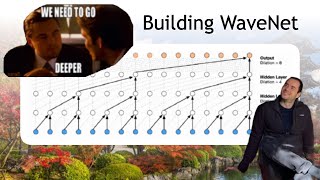

Andrej Karpathy: Tesla AI, Self-Driving, Optimus, Aliens, and AGI | Lex Fridman Podcast #333