The spelled-out intro to neural networks and backpropagation: building micrograd

In this segment of Andrej Karpathy's tutorial, he walks through the step‑by‑step construction of a minimal autograd engine (micrograd) and uses it to implement a multilayer perceptron (MLP). He starts by defining a Neuron class, showing how to compute a forward pass with a dot product, bias addition, and a non‑linearity. He then builds a Layer as a list of independent neurons and stacks Layers into an MLP that can handle arbitrary architectures. The video demonstrates a forward pass on a tiny binary‑classification dataset, introduces the mean‑squared‑error loss, and explains how backpropagation populates gradients on every parameter. Karpathy shows how to collect all parameters, perform a gradient‑descent update (including the sign convention), and iteratively improve the loss. He highlights a common bug – forgetting to zero gradients between iterations – and fixes it with a zerograd routine. The tutorial proceeds to a more realistic training loop with batching, learning‑rate decay, and L2 regularisation, and compares the micrograd implementation to PyTorch’s API (modules, parameters, backward, zerograd). Finally, he reflects on the broader significance of neural nets, emergent properties in large models, and how micrograd mirrors production‑grade libraries while remaining transparent. The segment ends with a brief look at how to register custom autograd functions in PyTorch.
Chapters
Hello, my name is Andrej Karpathy, and I've been training deep neural networks for a bit more than a decade. And in this lecture, I'd like to show you what neural network training looks like under the hood. So in particular, we are going to start with a blank Jupyter notebook, and by the end of this lecture, we will define and train a neural net, and you'll get to see everything that goes on under the hood and exactly sort of how that works on an intuitive level. Now specifically, what I would like to do is I would like to take you through building of micrograd. Now micrograd is this library that I released on GitHub about 2 years ago, but at the time I only uploaded the source code and you'd have to go in by yourself and really figure out how it works. So in this lecture I will take you through it step by step and kind of comment on all the pieces of it. So what is micrograd and why is it interesting? Micrograd is basically an autograd engine. Autograd is short for automatic gradient. And really what it does is it implements backpropagation. Now backpropagation is this algorithm that allows you to efficiently evaluate the gradient of some kind of a loss function with respect to the weights of a neural network. And what that allows us to do then is we can iteratively tune the weights of that neural network to minimize the loss function and therefore improve the accuracy of the network. So backpropagation would be at the mathematical core of any modern deep neural network library, like say PyTorch or JAX. So the functionality of micrograd is I think best illustrated by an example. So if we just scroll down here, you'll see that micrograd basically allows you to build out mathematical expressions. And here what we are doing is we have an expression that we're building out where you have two inputs, a and b, and you'll see that a and b are -4 and 2, but we are wrapping those values into this value object that we are going to build out as part of micrograd. So this value object will wrap the numbers themselves, and then we are going to build out a mathematical expression here where a and b are transformed into c, d, and eventually e, f, and g. And I'm showing some of the function— some of the functionality of micrograd and the operations that it supports. So you can add two value objects, you can multiply them, you you can raise them to a constant power, you can offset by 1, negate, squash at 0, square, divide by constant, divide by it, et cetera. And so we're building out an expression graph with these 2 inputs, a and b, and we're creating an output value of g. And micrograd will, in the background, build out this entire mathematical expression. So it will, for example, know that c is also a value, C was a result of an addition operation, and the child nodes of C are A and B, because the— and it will maintain pointers to A and B value objects. So we'll basically know exactly how all of this is laid out. And then not only can we do what we call the forward pass, where we actually look at the value of G— of course, that's pretty straightforward, we will access that using the.data attribute— and so the output of the forward pass the value of g is 24.7, it turns out. But the big deal is that we can also take this g value object and we can call.backward, and this will basically initialize backpropagation at the node g. And what backpropagation is going to do is it's going to start at g and it's going to go backwards through that expression graph, and it's going to recursively apply the chain rule from calculus. And what that allows us to do then is we're going to evaluate basically the derivative of g with respect to all the internal nodes like e, d, and c, but also with respect to the inputs a and b. And then we can actually query this derivative of g with respect to a. For example, that's a.grad. In this case, it happens to be 138. And the derivative of g with respect to b, which also happens to be here, 645. And this derivative, we'll see soon, is very important information because it's telling us how a and b are affecting g through this mathematical expression. So in particular, a.grad is 138. So if we slightly nudge a and make it slightly larger, 138 is telling us that g will grow, and the slope of that growth is going to be 138. And the slope of growth of b is going to be 645. So that's going to tell us about how g will respond if a and b get tweaked a tiny amount in a positive direction. Okay? Now you might be confused about what this expression is that we built out here. And this expression, by the way, is completely meaningless. I just made it up. I'm just flexing about the kinds of operations that are supported by Micrograd. What we actually really care about are neural networks. But it turns out that neural networks are just mathematical expressions. Just like this one, but actually slightly bit less crazy even. Neural networks are just a mathematical expression. They take the input data as an input, and they take the weights of a neural network as an input, and it's a mathematical expression, and the output are your predictions of your neural net or the loss function. We'll see this in a bit. But basically neural networks just happen to be a certain class of mathematical expressions. But backpropagation is actually significantly more general. It doesn't actually care about neural networks at all. It only cares about arbitrary mathematical expressions, and then we happen to use that machinery for training of neural networks. Now, one more note I would like to make at this stage is that, as you see here, Micrograd is a scalar-valued autograd engine. So it's working on the, you know, level of individual scalars like -4 and 2, and we're taking neural nets and we're breaking them down all the way to these atoms of individual scalars and all the little pluses and times, and it's just excessive. And so obviously you would never be doing any of this in production. It's really just for done for pedagogical reasons, because it allows us to not have to deal with these n-dimensional tensors that you would use in modern deep neural network library. So this is really done so that you understand and refactor out backpropagation and chain rule and understanding of neural network training. And then if you actually want to train bigger networks, you have to be using these tensors. But none of the math changes. This is done purely for efficiency. We are basically taking scalar value, uh, all the scalar values, we're packaging them up into tensors, which are just arrays of these scalars. And then because we have these large arrays, we're making operations on those large arrays that allows us to take advantage of the parallelism in a computer. And, uh, all those operations can be done in parallel, and then the whole thing runs faster. But really none of the math changes, and that's done purely for efficiency. So I don't think that it's pedagogically useful to be dealing with tensors from scratch, and I think— and that's why I fundamentally wrote micrograd, because you can understand how things work at the fundamental level and then you can speed it up later. Okay, so here's the fun part. My claim is that micrograd is what you need to train neural networks, and everything else is just efficiency. So you'd think that micrograd would be a very complex piece of code, and that turns out to not be the case. So if we just go to micrograd, and you'll see that there's only two files here in micrograd. This is the actual engine. It doesn't know anything about neural nets. And this is the entire neural nets library on top of micrograd. So engine and nn.py. So the actual backpropagation autograd engine that gives you the power of neural networks is literally 100 lines of code. Of like very simple Python, which we'll understand by the end of this lecture. And then nn.py, this neural network library built on top of the autograd engine, is like a joke. It's like we have to define what is a neuron, and then we have to define what is a layer of neurons, and then we define what is a multi-layer perceptron, which is just a sequence of layers of neurons. And so it's just a total joke. So basically, there's a lot of power that comes from only 150 lines of code, and that's all you need to understand to understand neural network training, and everything else is just efficiency. And of course, there's a lot to efficiency, but fundamentally that's all that's happening. Okay, so now let's dive right in and implement Micrograd step by step. The first thing I'd like to do is I'd like to make sure that you have a very good understanding intuitively of what a derivative is and exactly what information it gives you. So let's start with some basic imports that I copy-paste in every Jupyter Notebook always. And let's define the function, scalar-valued function, f(x) as follows. So I just made this up randomly. I just wanted a scalar-valued function that takes a single scalar x and returns a single scalar y. And we can call this function, of course, so we can pass in, say, 3.0 and get 20 back. Now we can also plot this function to get a sense of its shape. You can tell from the mathematical expression that this is probably a parabola, it's a quadratic. And so if we just create a set of scalar values that we can feed in using, for example, a range from -5 to 5 in steps of 0.25. So this is— so axis is just from -5 to 5, not including 5, in steps of 0.25. And we can actually call this function on this NumPy array as well. So we get a set of y's if we call f. On x's, and these y's are basically also applying, uh, function on every one of these elements independently. And we can plot this using matplotlib. So plt.plot(x's, y's), and we get a nice parabola. So previously here we fed in 3.0 somewhere here, and we received 20 back, which is here the y-coordinate. So now I'd like to think through what is the derivative of this function at any single input point x, right? So what is the derivative at different points x of this function? Now if you remember back to your calculus class, you've probably derived derivatives. So we take this mathematical expression 3x² 4x 5, and you would write out on a piece of paper and you would, you know, apply the product rule and all the other rules and derive the mathematical expression of the great derivative of the original function, and then you could plug in different x's and see what the derivative is. We're not going to actually do that because no one in neural networks actually writes out the expression for the neural net. It would be a massive expression. It would be, you know, thousands, tens of thousands of terms. No one actually derives the derivative, of course. And so we're not going to take this kind of like symbolic approach. Instead, what I'd like to do is I'd like to look at the definition of derivative and just make sure that we really understand what derivative is measuring, what it's telling you about the function. And so if we just look up derivative, we see that— okay, so this is not a very good definition of derivative. This is a definition of what it means to be differentiable. But if you remember from your calculus, it is the limit as h goes to 0 of f(x h) f(x) over h. So basically what it's saying is if you slightly bump up you're at some point x that you're interested in, or a, and if you slightly bump up, you know, you slightly increase it by small number h, how does the function respond? With what sensitivity does it respond? What is the slope at that point? Does the function go up or does it go down, and by how much? And that's the slope of that function, the slope of that response at that point. And so we can basically evaluate the derivative here numerically by taking a very small h. Of course, the definition would ask us to take h to 0. We're just going to pick a very small h, 0.001. And let's say we're interested in the point (3, 0). So we can look at f(x), of course, is 20. And now f(x h). So if we slightly nudge x in a positive direction, how is the function going to respond? And just looking at this, do you expect, do you expect f(x h) to be slightly greater than 20, or do you expect it to be slightly lower than 20? And since this 3 is here and this is 20, if we slightly go positively, the function will respond positively. So you'd expect this to be slightly greater than 20. And now by how much is telling you the sort of the strength of that slope, right? The size of that slope. So f(x+h) minus f(x), this is how much the function responded in the positive direction. And we have to normalize by the, run, so we have the rise over run to get the slope. So this of course is just a numerical approximation of the slope because we have to make age very, very small to converge to the exact amount. Now if I'm doing too many zeros, at some point I'm going to get an incorrect answer because we're using floating-point arithmetic and the representations of all these numbers in computer memory is finite, and at some point we get into trouble. So we can converge towards the right answer with this approach. But basically, at 3, the slope is 14, and you can see that by taking 3x² 4x 5 and differentiating it in our head. So 3x² would be 6x 4, and then we plug in x 3, so that's 18 4 is 14. So this is correct. So that's at 3. Now how about the slope at, say, -3? Would you expect— what would you expect for the slope? Now, telling the exact value is really hard, but what is the sign of that slope? So at -3, if we slightly go in the positive direction at x, the function would actually go down, and so that tells you that the slope would be negative. So we'll get a slight number below, uh, below 20. And so if we take the slope, we expect something negative. -22. Okay. And at some point here, of course, the slope would be 0. Now for this specific function, I looked it up previously, and it's at point 2/3. So at roughly 2/3, that's somewhere here, this derivative would be 0. So basically at that precise point, yeah, at that precise point, if we nudge in a positive direction, the function doesn't respond. This stays the same almost. And so that's why the slope is 0. Okay, now let's look at a bit more complex case. So we're going to start, you know, complexifying a bit. So now we have a function here with output variable d that is a function of 3 scalar inputs: a, b, and c. So a, b, and c are some specific values, 3 inputs into our expression graph, and a single output d. And so if we just print d, we get 4. And now what I'd like to do is I'd like to again look at the derivatives of d with respect to a, b, and c, and think through again just the intuition of what this derivative is telling us. So in order to evaluate this derivative, we're going to get a bit hacky here. We're going to again have a very small value of h, and then we're going to fix the inputs at some values that we're interested in. So these are the, the this is the point (a, b, c) at which we're going to be evaluating the derivative of D with respect to all a, b, and c at that point. So there's the inputs, and now we have d1 is that expression. And then we're going to, for example, look at the derivative of D with respect to a. So we'll take a and we'll bump it by h, and then we'll get d2 to be the exact same function. And now we're going to print, you know, font— f1, d1 is d1, d2 is d2, and print slope. So the derivative or slope here will be, of course, d2 minus d1 divided by h. So d2 minus d1 is how much the function increased when we bumped the, the specific input that we're interested in. By a tiny amount, and this is then normalized by h to get the slope. So, um, yeah, so this— so I just run this, we're going to print d1, uh, which we know is 4. Now d2 will be bumped, a will be bumped by h So let's just think through a little bit what d2 will be printed out here. In particular, d1 will be 4. Will d2 be a number slightly greater than 4 or slightly lower than 4? And that's going to tell us the, the sign of the derivative. So we're bumping a by h b is -3, c is 10. So you can just intuitively think through this derivative and what it's doing. a will be slightly more positive, and— but b is a negative number. So if a is slightly more positive, because b is -3, we're actually going to be adding less to d. So you'd actually expect that the value of the function would will go down. So let's just see this. Yeah, and so we went from 4 to 3.9996, and that tells you that the slope will be negative, and then will be a negative number because we went down, and then the exact number of slope will be— exact amount of slope is -3. And you can also convince yourself that -3 is the right answer mathematically and analytically because if you have a times b plus c and you are, you know, you have calculus, then differentiating a times b plus c with respect to a gives you just b. And indeed the value of b is negative 3, which is the derivative that we have. So you can tell that that's correct. So now if we do this with b, so if we bump b by a little bit in a positive direction, we'd get different slopes. So what is the influence of b on the output d? So if we bump b by a tiny amount in a positive direction, then because a is positive, we'll be adding more to d, right? So, and now what is the sensitivity? What is the slope of that addition? And it might not surprise you that this should be 2. And why is it 2? Because d of d by db, differentiating with respect to b, would give us a. And the value of a is 2. So that's also working well. And then if c gets bumped a tiny amount in h, by h, then of course a times b is unaffected, and now c becomes slightly bit higher. What does that do to the function? It makes it slightly bit higher because we're simply adding c, and it makes it slightly bit higher by the exact same amount that we added to c. And so that tells you that the slope is 1. That will be the the rate at which d will increase as we scale c. Okay, so we now have some intuitive sense of what this derivative is telling you about the function, and we'd like to move to neural networks. Now, as I mentioned, neural networks will be pretty massive expressions, mathematical expressions, so we need some data structures that maintain these expressions, and that's what we're going to start to build out now. So we're going to build out this value object that I showed you in the README page of micrograd. So let me copy-paste a skeleton of the first very simple value object. So class Value takes a single scalar value that it wraps and keeps track of, and that's it. So we can, for example, do value of 2.0, and then we can get— we can look at its content, and Python will internally use the wrapper function to return this string. Whoops, like that. So this is a value object with data equals 2 that we're creating here. Now we'd like to do is like, we'd like to be able to have not just like 2 values, but we'd like to do a plus b, right? We'd like to add them. So currently you would get an error because Python doesn't know how to add two value objects. So we have to tell it. So here's addition. So you have to basically use these special double underscore methods in Python to define these operators for these objects. So if we call the— if we use this plus operator, Python will internally call a.add(b). That's what will happen internally. And so b will be the other and self will be a. And so we see that what we're going to return is a new value object and it's just, it's going to be wrapping the plus of their data. But remember now, because data is the actual like numbered Python number, so this operator here is just the typical floating point plus addition now. It's not an addition of value objects. And will return a new value. So now a b should work and it should print value of -1 because that's 2 -3. There we go. Okay, let's now implement multiply just so we can recreate this expression here. So multiply, I think it won't surprise you, will be fairly similar. So instead of add, we're going to be using mul, and then here of course we want to do times. And so now we can create a c value object which will be 10.0. And now we should be able to do a times b. Well, let's just do a times b first. That's a value of -6 now. And by the way, I skipped over this a little bit. Suppose that I didn't have the repr function here, then it's just that you'll get some kind of an ugly expression. So what repr is doing is it's providing us a way to print out like a nicer looking expression in Python. So we don't just have something cryptic. We actually are, you know, it's a value of -6. So this gives us a `times`, and then this we should now be able to add `c` to it, because we've defined and told Python how to do `mul` and `add`. And so this will basically be equivalent to `a.mul(b)` and then this new value object will be `.add(c)`. And so let's see if that worked. Yep, so that worked well. That gave us 4, which is what we expect from bit4. And I believe we can just call them manually as well. There we go. So yeah. Okay, so now what we are missing is the connective tissue of this expression. As I mentioned, we want to keep these expression graphs, so we need to know and keep pointers about what values produce what other values. So here, for example, we are going to introduce a new variable which we'll call children, and by default it will be an empty tuple. And then we're actually going to keep a slightly different variable in the class which we'll call _prev which will be the set of children. This is how I done— I did it in the original micrograd looking at my code here. I can't remember exactly the reason, I believe it was efficiency, but this _children will be a tuple for convenience but then when we actually maintain it in the class it will be just this set. I believe for efficiency. So now when we are creating a value like this with a constructor, children will be empty and prev will be the empty set. But when we are creating a value through addition or multiplication, we're going to feed in the children of this value, which in this case is self and other. So those are the children here. So now we can do d.prev and we'll see that the children of d we now know are this value of -6 and value of 10. And this, of course, is the value resulting from a times b and the c value, which is 10. Now, the last piece of information we don't know— so we know now the children of every single value, but we don't know what operation created this value. So we need one more element here. Let's call it _up. And by default, this is the empty set for leaves. And then we'll just maintain it here. And now the operation will be just a simple string. And in the case of addition, it's plus, in the case of multiplication, it's times. So now we not just have d.pref, we also have a d.op. And we know that d was produced by an addition of those two values. And so now we have the full mathematical expression, and we're building out this data structure, and we know exactly how each value came to be, by what expression and from what other values. Now because these expressions are about to get quite a bit larger, we'd like a way to nicely visualize these expressions that we're building out. So for that, I'm going to copy-paste a bunch of slightly scary code that's going to visualize this, these expression graphs for us. So here's the code, and I'll explain it in a bit. But first, let me just show you what this code does. Basically what it does is it creates a new function draw_dot that we can call on some root node and then it's going to visualize it. So if we call draw_dot on d, which is this final value here that is a times b plus c, it creates something like this. So this is d and you see that this is a times b creating an intermediate value plus c gives us this output node d. So that's draw_dot of d and I'm not going to go through this in complete detail. You can take a look at Graphviz and its API. Graphviz is an open-source graph visualization software, and what we're doing here is we're building out this graph in Graphviz API. And you can basically see that trace is this helper function that enumerates all of the nodes and edges in the graph. So that just builds a set of all the nodes and edges, and then we iterate through all the nodes and we create special node objects for them in using.node, and then we also create edges using..edge. And the only thing that's like slightly tricky here is you'll notice that I basically add these fake nodes, which are these operation nodes. So for example, this node here is just like a plus node, and I create these special op nodes here, and I connect them accordingly. So these nodes of course are not actual nodes in the original graph. They're not actually a value object. The only value objects here are the things in squares. Those are actual value objects or representations thereof. And these op nodes are just created in this draw routine so that it looks nice. Let's also add labels to these graphs just so we know what variables are where. So let's create a special _label or let's just do label equals empty by default and save it in each node. And then here we're going to do label is A, label is B, label is C. And then let's create a special equals A times B. And e.label will be e. It's kind of naughty. And e will be e c, and d.label will be d. Okay, so nothing really changes. I just added this new e function, a new e variable. And then here, when we are printing this, I'm going to print the label here. So this will be a %s bar, and this will be n.label. And so now we have the label on the lot here. So this is A, B creating E, and then E plus C creates D, just like we have it here. And finally, let's make this expression just one layer deeper. So D will not be the final output node. Instead, after D, we are going to create a new value object called f. We're going to start running out of variables soon. f will be -2.0, and its label will of course just be f. And then L, capital L, will be the output of our graph, and L will be d times f. Okay, so L will be -8 as the output. So now we don't just draw a d, we draw L. Okay, and somehow the label of L was undefined. Oops, L.label has to be explicitly sort of given to it. There we go. So L is the output. So let's quickly recap what we've done so far. We are able to build out mathematical expressions using only plus and times so far. They are scalar valued along the way, and we can do this forward pass and build out a mathematical expression. So we have multiple inputs here, a, b, c, and f, going into a mathematical expression that produces a single output, l. And this here is visualizing the forward pass. So the output of the forward pass is -8. That's the value. Now what we'd like to do next is we'd like to run backpropagation. And in backpropagation, we are going to start here at the end and we're going to reverse and calculate the gradient along, along all these intermediate values. And really what we're computing for every single value here, we're going to compute the derivative of that node with respect to L. So the derivative of L with respect to L is just 1, and then we're going to derive— what is the derivative of L with respect to f, with respect to d, with respect to c? With respect to e, with respect to b, and with respect to a. And in a neural network setting, you'd be very interested in the derivative of basically this loss function L with respect to the weights of a neural network. And here, of course, we have just these variables a, b, c, and f, but some of these will eventually represent the weights of a neural net. And so we'll need to know how those weights are impacting the loss function. So we'll be interested basically in the derivative of the output with respect to some of its leaf nodes, and those leaf nodes will be the weights of the neural net. And the other leaf nodes, of course, will be the data itself. But usually we will not want or use the derivative of the loss function with respect to data because the data is fixed, but the weights will be iterated on using the gradient information. So next, we are going to create a variable inside the Value class that maintains the derivative of L with respect to that value, and we will call this variable grad. So there is a.data and there's a self.grad, and initially it will be 0. And remember that 0 basically means no effect. So at initialization, we're assuming that every value does not impact, does not affect the output, right? Because if the gradient is 0, that means that changing this variable is not changing the loss function. So by default, we assume that the gradient is 0, and then now that we have grad and it's, you know, 0.0, we are going to be able to visualize it here after data. So here grad is 0.4f, and this will be in that grad. And now we are going to be showing both the data and the grad. Initialized at 0, and we are just about getting ready to calculate the backpropagation. And of course, this grad, again, as I mentioned, is representing the derivative of the output, in this case L, with respect to this value. So with respect to— so this is the derivative of L with respect to f, with respect to d, and so on. So let's now fill in those gradients and actually do backpropagation manually. So let's start filling in these gradients and start all the way at the end, as I mentioned here. First, we are interested to fill in this gradient here. So what is the derivative of L with respect to L? In other words, if I change L by a tiny amount h, how much does L change? It changes by h, so it's proportional, and therefore derivative will be 1. We can of course measure these or estimate these numerical gradients numerically, just like we've seen before. So if I take this expression and I create a def lol function here and put this here. Now the reason I'm creating a gating function lol here is because I don't want to pollute or mess up the global scope here. This is just kind of like a little staging area, and as you know in Python, all of these will be local variables to this function, so I'm not changing any of the global scope here. So here l1 will be l, and then copy pasting this expression We're going to add a small amount h in, for example, a, right? And this would be measuring the derivative of L with respect to a. So here, this will be L2, and then we want to print that derivative. So print L2 minus L1, which is how much L changed, and then normalize it by h. So this is the rise over run. And we have to be careful because L is a value node, so we actually want its data, um, so that these are floats, divided by h. And this should print the derivative of L with respect to a, because a is the one that we bumped a little bit by h. So what is the derivative of L with respect to a? It's 6. Okay, and obviously if we change L by h, then that would be here. Effectively, um, this looks really awkward, but changing L by h, you see the derivative here is 1. Um, that's kind of like the base case of what we are doing here. So basically we can come up here and we can manually set L.grad to 1. This is our manual backpropagation. L.grad is 1, and let's redraw, and we'll see that we filled in grad is 1 for l. We're now going to continue the backpropagation. So let's here look at the derivatives of l with respect to d and f. Let's do d first. So what we are interested in, if I create a Markdown note here, is we'd like to know— basically we have that l is d times f, and we'd like to know what is dl/dt. What is that? And if you know your calculus, uh, L is d times f. So what is dL/dD? It would be f. And if you don't believe me, we can also just derive it because the proof would be fairly straightforward. We go to the definition of the derivative, which is f(x h) f(x) h, as a limit, limit of h goes to 0, of this kind of expression. So when we have L is D times f, then increasing D by h would give us the output of D plus h times f. That's basically f of x plus h, right? Minus D times f, and then divide h. And symbolically expanding out here, we would have basically D times f plus h times f minus D times f divide h. And then you see how the Df minus Df cancels, so you're left with h times f. F divided by h, which is f. So in the limit as h goes to 0 of, you know, derivative definition, we just get f in the case of d times f. So symmetrically, dL/df will just be d. So what we have is that f.grad, we see now, is just the value of d, which is 4. And we see that d.grad is just the value of f, and so the value of f is -2. So we'll set those manually. Let me erase this markdown node, and then let's redraw what we have. Okay, and let's just make sure that these were correct. So we seem to think that dl/dt is -2, so let's double-check. Um, let me erase this +h from before, and now we want the derivative with respect to f. So let's just come here when I create f, and let's do a +h here, and this should print the derivative of L with respect to f. So we expect to see 4. Yeah, and this is for up to floating point funkiness. And then dl by dd should be f, which is negative 2. Grad is negative 2. So if we again come here and we change d, d.data plus equals h right here. So we expect, so we've added a little h and then we see how l changed. And we expect to print -2. There we go. So we've numerically verified. What we're doing here is kind of like an inline gradient check. Gradient check is when we are deriving this like backpropagation and getting the derivative with respect to all the intermediate results. And then numerical gradient is just estimating it using small step size. Now we're getting to the crux of backpropagation. So this will be the most important node to understand, because if you understand the gradient for this node, you understand all of backpropagation and all of training of neural nets, basically. So we need to derive dl/dc. In other words, the derivative of L with respect to C, because we've computed all these other gradients already. Now we're coming here and we're continuing the backpropagation. Manually. So we want dl/dC, and then we'll also derive dl/dE. Now here's the problem. How do we derive dl/dC? We actually know the derivative of L with respect to D, so we know how L is sensitive to D. But how is L sensitive to C? So if we wiggle C, how does that impact L through D? So we know dl/dc, and we also here know how c impacts d. And so just very intuitively, if you know the impact that c is having on d and the impact that d is having on l, then you should be able to somehow put that information together to figure out how c impacts l. And indeed, this is what we can actually do. So in particular, we know, just concentrating on d first, let's look at how what is the derivative basically of D with respect to C? So in other words, what is dD/dC? So here we know that D is C times C plus E. That's what we know. And now we're interested in dD/dC. If you just know your calculus again and you remember that differentiating C plus E with respect to C, you know that that gives you 1.0. And we can also go back to the basics and derive this. Because again, we can go to our f(x h) f(x) divided by h. That's the definition of a derivative as h goes to 0. And so here, focusing on c and its effect on d, we can basically do the f(x h) will be c is incremented by h plus e. That's the first evaluation of our function minus c plus e, and then divide h. And so what is this? Uh, just expanding this out, this will be c h e c e h. And then you see here how c c cancels, e e cancels, we're left with h h which is 1.0. And so by symmetry also, d/dE will be 1.0 as well. So basically the derivative of a sum expression is very simple, and, and this is the local derivative. So I call this the local derivative because we have the final output value all the way at the end of this graph, and we're now like a small node here, and this is a little plus node, and it— the little plus node doesn't know anything about the rest of the graph that it's embedded in. All it knows is that it did a plus. It took a c and an e, added them, and created d. And this plus node also knows the local influence of c on d, or rather, rather, the derivative of d with respect to c. And it also knows the derivative of D with respect to E. But that's not what we want, that's just a local derivative. What we actually want is dL by dC, and L could— L is here just one step away, but in a general case, this little plus node could be embedded in like a massive graph. So again, we know how L impacts D, and now we know how C and E impact D. How do we put that information together to write dL by dC? And the answer of course is the chain rule in calculus. And so I pulled up chain rule here from Wikipedia and I'm going to go through this very briefly. So chain rule— Wikipedia sometimes can be very confusing and calculus can, can be very confusing. Like this is the way I learned chain rule and it was very confusing. Like what is happening? It's just complicated. So I like this expression much better. If a variable z depends on a variable y, which itself depends on a variable x, then z depends on x as well, obviously, through the intermediate variable y. And in this case, the chain rule is expressed as: if you want dz/dx, then you take the dz/dy and you multiply it by dy/dx. So the chain rule fundamentally is telling you how we chain these, uh, derivatives together correctly. So to differentiate through a function composition, we have to apply a multiplication of those derivatives. So that's really what chain rule is telling us. And there's a nice little intuitive explanation here which I also think is kind of cute. The chain rule states that knowing the instantaneous rate of change of z with respect to y y relative to x allows one to calculate the instantaneous rate of change of z relative to x as a product of those two rates of change, simply the product of those two. So here's a good one: if a car travels twice as fast as a bicycle and the bicycle is four times as fast as a walking man, then the car travels two times four, eight times as fast as the man. And so this makes it very clear that the correct thing to do, sort of is to multiply. So car is twice as fast as bicycle, and bicycle is 4 times as fast as man, so the car will be 8 times as fast as the man. And so we can take these intermediate rates of change, if you will, and multiply them together, and that justifies the chain rule intuitively. So have a look at chain rule, but here really what it means for us is there's a very simple recipe for deriving what we want, which is dl/dc. And what we have so far is we know want, and we know what is the impact of d on L. So we know dL/dt, the derivative of L with respect to dt, we know that that's -2. And now because of this local reasoning that we've done here, we know dL/dt. So how does c impact d? And in particular, this is a plus node, so the local derivative is simply 1.0. It's very simple. And so the chain rule tells us that dl/dc going through this intermediate variable will just be simply dl/dd times dd/dc. That's chain rule. So this is identical to what's happening here, except z is our L, y is our D, and x is our C. So we literally just have to multiply these. And because these local derivatives like dd/dc are just 1, we basically just copy over dl/dd because this is just times 1. So what is it? So because dl/dt is -2, what is dl/dc? Well, it's the local gradient, 1.0, times dl/dt, which is -2. So literally what a plus node does, you can look at it that way, is it literally just routes the gradient because the plus node's local derivatives are just 1. And so in the chain rule, 1 times dl/dt is, um, is, uh, it's just ��L/��D. And so that derivative just gets routed to both C and to E in this case. So basically, um, we have that E.grad— or let's start with C since that's the one we've looked at— is -2 times 1, -2. And in the same way, by symmetry, E.grad will be -2. That's the claim. So we can set those, we can redraw, and you see how we just assigned -2, -2. So this backpropagating signal, which is carrying the information of like what is the derivative of L with respect to all the intermediate nodes, we can imagine it almost like flowing backwards through the graph, and a plus node will simply distribute the derivative to all the leaf nodes— sorry, to all the children nodes of it. So this is the claim, and now let's verify it. So let me remove the plus H here from before, and now instead what we want to do is we want to increment C. So C.data will be incremented by H, and when I run this, we expect to see negative 2. Negative 2. And then of course for E, so E.data plus equals H, and we expect to see negative 2. Simple. So those are the derivatives of these internal nodes, and now we're going to recurse our way backwards again, and we're again going to apply the chain rule. So here we go, our second application of chain rule, and we will apply it all the way through the graph. We just happen to only have one more node remaining. We have that dL/dE, as we have just calculated, is -2. So we know that. So we know the derivative of L with respect to e. And now we want dL/dA, right? And the chain rule is telling us that that's just dL/dE, negative 2, times the local gradient. So what is the local gradient? Basically dE/dA. We have to look at that. So I'm a little times node inside a massive graph. And I only know that I did a times b and I produced an e. So now what is dE/dA and dE/dB? That's the only thing that I sort of know about. That's my local gradient. So because we have that e is a times b, we're asking what is dE/dA? And of course, we just did that here. We had a times, so I'm not going to re-drive it. But if you want to differentiate this with respect to a, you'll just get b, right? The value of b, which in this case is -3.0. So basically, we have that dl/da. Well, let me just do it right here. We have that a.grad, and we are applying chain rule here. Is dl/dE, which we see here is -2, times— what is dE/dA? It's the value of B, which is -3. That's it. And then we have B dot grad is again dl/dE, which is -2, just the same way, times— what is dE/dA? Db is the value of a, which is 2.0. That's the value of a. So these are our claimed derivatives. Let's redraw. And we see here that a.grad turns out to be 6 because that is -2 times -3, and b.grad is -4 times— sorry, is -2 times 2. Which is -4. So those are our claims. Let's delete this and let's verify them. We have a here, a.data h. So the claim is that a.grad is 6. Let's verify, 6. And we have b.data h. So nudging b by h, and looking at what happens, we claim it's -4, and indeed it's -4 plus minus again float oddness. And that's it. This, that was the manual backpropagation all the way from here to all the leaf nodes. And we've done it piece by piece. And really all we've done is, as you saw, we iterated through all the nodes one by one and locally apply the chain rule. We always know what is the derivative of L with respect to this little output, and then we look at how this output was produced. This output was produced through some operation, and we have the pointers to the children nodes of this operation. And so in this little operation, we know what the local derivatives are, and we just multiply them onto the derivative always. So we just go through and recursively multiply on the local derivatives. And that's what backpropagation is, is just a recursive application of chain rule backwards through the computation graph. Let's see this power in action just very briefly. What we're going to do is we're going to nudge our inputs to try to make L go up. So in particular, what we're doing is we want a.data, we're going to change it. And if we want L to go up, that means we just have to go in the direction of the gradient. So a should increase in the direction of gradient by like some small step amount. This is the step size, and we don't just want this for b, but also for b, also for c, also for f. Those are leaf nodes which we usually have control over, and if we nudge in direction of the gradient, we expect a positive influence on L. So we expect L to go up positively. So it should become less negative. It should go up to say negative, you know, 6 or something like that. It's hard to tell exactly, and we'd have to rerun the forward pass. So let me just do that here. This would be the forward pass. F would be unchanged. This is effectively the forward pass. And now if we print l.data, we expect— because we nudged all the values, all the inputs in the direction of gradient, we expected less negative L. We expect it to go up. So maybe it's -6 or so. Let's see what happens. Okay, -7. And this is basically one step of an optimization that we'll end up running. And really this gradient just gives us some power because we know how to influence the final outcome. And this will be extremely useful for training neural nets, as we'll soon see. So now I would like to do one more example of manual backpropagation using a bit more complex and useful example. We are going to backpropagate through a neuron. So we want to eventually build out neural networks, and in the simplest case, these are multilayer perceptrons, as they're called. So this is a two-layer neural net. And it's got these hidden layers made up of neurons, and these neurons are fully connected to each other. Now biologically, neurons are very complicated devices, but we have very simple mathematical models of them. And so this is a very simple mathematical model of a neuron. You have some inputs, x's, and then you have these synapses that have weights on them. So the w's are weights, and then the synapse interacts with the input to this neuron multiplicatively. So what flows to the cell body of this neuron is W times X, but there's multiple inputs, so there's many W times Xs flowing into the cell body. The cell body then has also like some bias, so this is kind of like the inner innate sort of trigger happiness of this neuron. So this bias can make it a bit more trigger happy or a bit less trigger happy regardless of the input. But basically we're taking all the w times x of all the inputs, adding the bias, and then we take it through an activation function. And this activation function is usually some kind of a squashing function, like a sigmoid or tanh or something like that. So as an example, we're going to use the tanh in this example. NumPy has a np.tanh, so we can call it on a range and we can plot it. This is the tanh function, and you see that the inputs as they come in get squashed on the y-coordinate here. So, um, right at 0, we're going to get exactly 0, and then as you go more positive in the input, then you'll see that the function will only go up to 1 and then plateau out. And so if you pass in very positive inputs, we're going to cap it smoothly at 1, and on the negative side we're going to cap it smoothly to -1. So that's tanh, and that's the squashing function or an activation function. And what comes out of this neuron is just the activation function applied to the dot product of the weights and the inputs. So let's write one out. I'm going to copy paste because I don't want to type too much, but okay, so here we have the inputs x1, x2. So this is a 2-dimensional neuron, so 2 inputs are going to come in. These are thought of as the weights of this neuron, weights w1, w2, and these weights again are the synaptic strengths for each input. And this is the bias of the neuron, b. And now what we want to do is, according to this model, we need to multiply x1 times w1 and x2 times w2, and then we need to add bias on top of it. And it gets a little messy here, but all we are trying to do is x1 w1 plus x2 w2 plus b, and these are multiplied here, except I'm doing it in small steps so that we actually have pointers to all these intermediate nodes. So we have x1 w1 variable, x times x2 w2 variable, and I'm also labeling them. So n is now the cell body raw, raw activation without the activation function for now. And this should be enough to basically plot it. So draw_dot of n gives us x1 times w1, x2 times w2 being added, then the bias gets added on top of this. And this n is this sum. So we're now going to take it through an activation function, and let's say we use the tanh so that we produce the output. So what we'd like to do here is we'd like to do the output, and I'll call it o, is, um, n.tanh. Okay, but we haven't yet written the tanh. Now the reason that we need to implement another tanh function here is that tanh is a hyperbolic function, and we've only so far implemented a plus and a times, and you can't make a tanh out of just pluses and times. You also need exponentiation. So tanh is this kind of a formula here. You can use either one of these, and you see that there is exponentiation involved, which we have not implemented yet for our little value node here. So we're not going to be able to produce tanh yet, and we have to go back up and implement something like it. Now one option here is we could actually implement exponentiation, right? And we could return the exp of a value instead of a tanh of a value. Because if we had exp, then we have everything else that we need. So because we know how to add and we know how to— we know how to add and we know how to multiply, so we'd be able to create tanh and if we knew how to exp. But for the purposes of this example, I specifically wanted to show you that we don't necessarily need to have the most atomic pieces in, in this value object. We can actually like create functions at arbitrary points of abstraction. They can be complicated functions, but they can be also very, very simple functions like a plus. And it's totally up to us. The only thing that matters is that we know how to differentiate through any one function. So we take some inputs and we make an output. The only thing that matters, it can be arbitrarily complex function as long as you know how to create the local derivative. If you know the local derivative of how the inputs impact the output, then that's all you need. So we're going to cluster up all of this expression and we're not going to break it down to its atomic pieces. We're just going to directly implement tanh. So let's do that. def tanh, and then out will be a value. Of, and we need this expression here, so let me actually copy paste. Let's grab n, which is self.theta, and then this I believe is the tanh. Math.exp of 2, no, n, n 1 over 2n 1. Maybe I can call this x, just so that it matches exactly. Okay, and now this will be t, and children of this node, there's just one child, and I'm wrapping it in a tuple. So this is a tuple of one object, just self, and here the name of this operation will be tenh, and we're going to return that. Okay, so now value should be implementing tanh, and now we can scroll all the way down here and we can actually do n.tanh, and that's going to return the tanh'd output of n. And now we should be able to draw a dot of o, not of n. So let's see how that worked. There we go. And went through tanh to produce this output. So now tanh is a sort of our little micrograd-supported node here as an operation. And as long as we know the derivative of tanh, then we'll be able to backpropagate through it. Now let's see this tanh in action. Currently it's not squashing too much because the input to it is pretty low. So if the bias was increased, to say 8, then we'll see that what's flowing into the tanh now is 2, and tanh is squashing it to 0.96. So we're already hitting the tail of this tanh, and it will sort of smoothly go up to 1 and then plateau out over there. Okay, so now I'm going to do something slightly strange. I'm going to change this bias from 8 to this number, 6.88, etc., and I'm going to do this for specific reasons because we're We're about to start backpropagation, and I want to make sure that our numbers come out nice. They're not like very crazy numbers. They're nice numbers that we can sort of understand in our head. Let me also add o's label. o is short for output here. So that's the o. Okay, so 0.88 flows into tanh, comes out 0.7, so on. So now we're going to do backpropagation, and we're going to fill in all the gradients. So what is the derivative of O with respect to all the inputs here? And of course, in a typical neural network setting, what we really care about the most is the derivative of these neurons on the weights, specifically the w2 and w1, because those are the weights that we're going to be changing in part of the optimization. And the other thing that we have to remember is here we have only a single neuron, but in the neural net you typically have many neurons and they're connected. So this is only like a one small neuron, a piece of a much bigger puzzle, and eventually there's a loss function that sort of measures the accuracy of the neural net, and we're backpropagating with respect to that accuracy and trying to increase it. So let's start off backpropagation here, and what is the derivative of O with respect to O? The base case sort of we know always is that the gradient is just 1.0. So let me fill it in. And then let me split out the drawing function here. And then here, cell, clear this output here. Okay. So now when we draw O, we'll see that, oh, that grad is 1. So now we're going to backpropagate through the tanh. So to backpropagate through tanh, we need to know the local derivative. Tanh. So if we have that O is tanh of n, then what is dO/dn? Now what you could do is you could come here and you could take this expression and you could do your calculus derivative taking, and that would work. But we can also just scroll down Wikipedia here into a section that puts hopefully tells us that derivative, uh, d/dx of tanh(x) is any of these. I like this one, 1 tanh²(x). So this is 1 tanh(x)². So basically what this is saying is that dO/dn is 1 tanh(n)². And we already have tanh(n), it's just O, so it's 1 minus O squared. So O is the output here. So the output is this number, O.data is this number, and then what this is saying is that dO/dn is 1 minus this squared, so 1 minus O.data squared is 0.5 conveniently. So the local derivative of this tanh operation here is 0.5. And so that would be dO/dn. So we can fill in that n.grad is 0.5. We'll just fill it in. So this is exactly 0.5, one half. So now we're going to continue the backpropagation. This is 0.5 and this is a plus node. So how is backprop going to— what is backprop going to do here? And if you remember our previous example, a plus is just a distributor of gradient. So this gradient will simply flow to both of these equally. And that's because the local derivative of this operation is 1. For every one of its nodes. So 1 times 0.5 is 0.5. So therefore we know that this node here, which we called this, its grad is just 0.5. And we know that b.grad is also 0.5. So let's set those and let's draw. So those are 0.5. Continuing, we have another plus. 0.5 again will just distribute So 0.5 will flow to both of these. So we can set theirs, x2w2 as well, that grad is 0.5 as well. And let's redraw. Pluses are my favorite operations to backpropagate through because it's very simple. So now what's flowing into these expressions is 0.5. And so really, again, keep in mind what derivative is telling us at every point in time along along here. This is saying that if we want the output of this neuron to increase, then the influence on these expressions is positive on the output. Both of them are positive contribution to the output. So now backpropagating to x2 and w2 first, this is a times node, so we know that the local derivative is, you know, the other term, and So if we want to calculate x2.grad, then can you think through what it's going to be? So x2.grad will be w2.data times this x2.w2.grad, right? And w2.grad will be x2.data times x2.w2.grad, right? So that's the little local piece of chain rule. Let's set them and let's redraw. So here we see that the gradient on our weight 2 is 0 because x2's data was 0, right? But x2 will have the gradient 0.5 because data here was 1. And so what's interesting here, right, is because the input x2 was 0, then because of the way the times works, of course this gradient will be 0. And think about intuitively why that is. Derivative always tells us the influence of this on the final output. If I wiggle w2, how is the output changing? It's not changing because we're multiplying by 0. So because it's not changing, there is no derivative. And 0 is the correct answer because we're squashing that 0. And let's do it here. 0.5 should come here and flow through this times. And so we'll have that x1.grad is— can you think through a little bit what this should be? The local derivative of times with respect to x1 is going to be w1. So w1's data times— x1 w1.grad, and w1.grad will be x1.data times x1 w2— w1.grad. Let's see what those came out to be. So this is 0.5, so this would be -1.5, and this would be 1. And we've backpropagated through this expression. These are the actual final derivatives. So if we want this neuron's output to increase, we know that what's necessary is that, uh, w2— we have no gradient, w2 doesn't actually matter to this neuron right now, but this neuron, this weight should go up. So if this weight goes up, then this neuron's output would have gone up, and proportionally because the gradient is 1. Okay, so doing the backpropagation manually is obviously ridiculous, so we are now going to put an end to this suffering. And we're going to see how we can implement the backward pass a bit more automatically. We're not going to be doing all of it manually out here. It's now pretty obvious to us by example how these pluses and times are backpropagating gradients. So let's go up to the value object and we're going to start codifying what we've seen in the examples below. So we're going to do this by storing a special self.backward. And this will be a function which is going to do that little piece of chain rule at each little node that compute— that took inputs and produced output. We're going to store how we are going to chain the outputs gradient into the inputs gradients. So by default, this will be a function that doesn't do anything. So And you can also see that here in the value in micrograd. So we have this backward function by default doesn't do anything. This is an empty function. And that would be sort of the case, for example, for a leaf node. For a leaf node, there's nothing to do. But now if when we're creating these out values, these out values are an addition of self and other. And so we will want to set out's backward to be the function that propagates the gradient. So let's define what should happen, and we're going to store it in a closure. Let's define what should happen when we call outgrad. For addition, our job is to take outgrad and propagate it into some self.grad and other.grad. So basically, we want to set self.grad to something, and we want to set other.grad to something. Okay. And the way we saw below how chain rule works, we want to take the local derivative times the sort of global derivative, I should call it, which is the derivative of the final output of the expression with respect to out.data. With respect to out. So the local derivative of self in an addition is 1.0. So it's just 1.0 times out's grad. That's the chain rule. And others.grad will be 1.0 times out.grad. And what you— basically what you're seeing here is that out's grad will simply be copied onto self's grad and others' grad. As we saw happens for an addition operation. So we're going to later call this function to propagate the gradient having done an addition. Let's now do multiplication. We're going to also define @backward and we're going to set its backward to be backward and we want to chain out_grad into self.grad and others.grad. And this will be a little piece of chain rule for multiplication. So we'll have— so what should this be? Can you think through? So what is the local derivative here? The local derivative was others.data and then— oops, others.data and then times outgrad. That's chain rule. And here we have self.data times out.grad. That's what we've been doing. And finally here for tanh, that backward, and then we want to set out.backward to be just backward. And here we need to backpropagate. We have out.grad and we want to chain it into self.grad. And salt.grad will be the local derivative of this operation that we've done here, which is tanh. And so we saw that the local gradient is 1 minus the tanh of x squared, which here is t. That's the local derivative because that's— t is the output of this tanh. So 1 minus t squared is the local derivative. And then gradient has to be multiplied because of the chain rule. So aux.grad is chained through the local gradient into salt.grad. And that should be basically it. So we're going to redefine our value node. We're going to swing all the way down here and we're going to redefine our expression, make sure that all the grads are zero. Okay, but now we don't have to do this manually anymore. We are going to basically be calling the.backward in the right order. So first we want to call o.backward. So o was the outcome of tanh, right? So colon o.backward will be this function. This is what it will do. Now we have to be careful because there's a times out.grad, and out.grad, remember, is initialized to 0. So here we see grad 0. So as a base case, we need to set auth.grad to 1.0 to initialize this with 1, and then once this is 1, we can call o.backward, and what that should do is it should propagate this grad through tanh. So the local derivative times the global derivative, which is initialized at 1, so this should— um, uh, doh. So I thought about redoing it, but I figured I should just leave the error in here because it's pretty funny. Why is numpy.object not callable? It's because I screwed up. We're trying to save these functions, so this is correct. This here, you don't want to call the function because that returns None. These functions return None. We just want to store the function. So let me redefine the value object, and then we're going to come back in, redefine the expression draw_dot. Everything is great. O.grad is 1, o.grad is 1. And now, now this should work, of course. Okay, so all that backward should have— this grad should now be 0.5 if we redraw. And if everything went correctly, 0.5. Yay! Okay, so now we need to call ans.backwards. So that seems to have worked. So n.backward routed the gradient to both of these. So this is looking great. Now we can of course call b.backward. What's going to happen? Well, b doesn't have a backward. b.backward, because b is a leaf node, b.backward is by initialization the empty function, so nothing would happen, but we can call it on it. But when we call this one, it's backward, then we expect this 0.5 to get further routed, right? So there we go, 0.5, 0.5. And then finally we want to call it here on x2, w2. And on x1, w1. Let's do both of those, and there we go. So we get 0, 0.5, -1.5, and 1, exactly as we did before. But now we've done it through calling.backward sort of manually. So we have the one last piece to get rid of, and which is us calling _backward manually. So let's think through what we are actually doing. We've laid out a mathematical expression and now we're trying to go backwards through that expression. So going backwards through the expression just means that we never want to call a.backward for any node before we've done sort of everything after it. So we have to do everything after it before we're ever going to call.backward on any one node. We have to get all of its full dependencies everything that it depends on has to propagate to it before we can continue backpropagation. So this ordering of graphs can be achieved using something called topological sort. So topological sort is basically a laying out of a graph such that all the edges go only from left to right, basically. So here we have a graph, it's a directed acyclic graph, a DAG. And this is two different topological orders of it, I believe, where basically you'll see that it's laying out of the nodes such that all the edges go only one way, from left to right. And implementing topological sort, you can look in Wikipedia and so on. I'm not going to go through it in detail. But basically, this is what builds a topological graph. We maintain a set of visited nodes, And then we are going through starting at some root node, which for us is O. That's where we want to start the topological sort. And starting at O, we go through all of its children, and we need to lay them out from left to right. And basically, this starts at O. If it's not visited, then it marks it as visited. And then it iterates through all of its children and calls build_topological on them. And then after it's gone through all the children, it adds itself. So basically, this node that we're going to call it on, like say O, is only going to add itself to the topo list after all of the children have been processed. And that's how this function is guaranteeing that you're only going to be in the list once all your children are in the list. And that's the invariant that is being maintained. So if we built topo on O, and then inspect this list, we're going to see that it ordered our value objects. And the last one is the value of 0.707, which is the output. So this is O, and then this is N, and then all the other nodes get laid out before it. So that builds the topological graph. And really what we're doing now is we're just calling.backward. On all of the nodes in a topological order. So if we just reset the gradients, they're all 0. What did we do? We started by setting o.grad to be 1. That's the base case. Then we built a topological order, and then we went for node in reversed of topo. Now in the reverse order, because this list goes from, you know, we need to go through it in reversed order. So starting at o, node.backward, and this should be it. There we go. Those are the correct derivatives. Finally, we are going to hide this functionality. So I'm going to copy this and we're going to hide it inside the value class because we don't want to have all that code lying around. So instead of an underscore backward, we're now going to define an actual backward, so that backward without the underscore, and that's going to do all the stuff that we just derived. So let me just clean this up a little bit. So we're first going to build the topological graph starting at self. So build_topo of self will populate the topological order into the topo list, which is a local variable. Then we set self.grad to be 1, and then for each node in the reversed list, so starting at us and going to all the children, uh, underscore backward And that should be it. So save, come down here, redefine. Okay, all the grads are 0. And now what we can do is o.backward without the underscore, and there we go. And that's, that's backpropagation, at least for one neuron. We shouldn't be too happy with ourselves actually, because we have a bad bug and we have not surfaced the bug because of some specific conditions that we are— we have to think about right now. So here's the simplest case that shows the bug. Say I create a single node A and then I create a B that is A A and then I call backward. So what's going to happen is a is 3, and then a is b is a plus a. So there's two arrows on top of each other here. Then we can see that b is, of course, the forward pass works. b is just a plus a, which is 6. But the gradient here is not actually correct that we calculated automatically. And that's because Of course, just doing calculus in your head, the derivative of b with respect to a should be 2, 1 1. It's not 1. Intuitively, what's happening here, right? So b is the result of a a, and then we called backward on it. So let's go up and see what that does. b is a result of addition. So out as b. And then when we called backward, what happened is self.grad was set to 1, and then other.grad was set to 1. But because we're doing a a, self and other are actually the exact same object. So we are overriding the gradient. We are setting it to 1, and then we are setting it again to 1, and that's why it stays at 1. So that's a problem. There's another way to see this in a little bit more complicated expression. So here we have a and b, and then, uh, d will be the multiplication of the two and e will be the addition of the two. And then we multiply e times d to get f, and then we call it f.backward And these gradients, if you check, will be incorrect. So fundamentally what's happening here again is, um, basically we're going to see an issue anytime we use a variable more than once. Until now in these expressions above, every variable is used exactly once, so we didn't see the issue. But here, if a variable is used more than once, what's going to happen during backward pass? We're backpropagating from f to e to d, so far so good, but now E calls backward and it deposits its gradients to A and B, but then we come back to D and call backward and it overwrites those gradients at A and B. So that's obviously a problem. And the solution here, if you look at the multivariate case of the chain rule and its generalization there, the solution there is basically that we have to accumulate these gradients, these gradients add. And so instead of setting those gradients, we can simply do We need to accumulate those gradients. And this will be okay, remember, because we are initializing them at 0. So they start at 0, and then any contribution that flows backwards will simply add. So now if we redefine this one, because the this now works because a.grad started at 0, and when we called b.backward, we deposit 1, and then we deposit 1 again, and now this is 2, which is correct. And here this will also work, and we'll get correct gradients because when we call e.backward, we will deposit the gradients from this branch and then we get to back— to d.backward, it will deposit its own gradients, and then those gradients simply add on top of each other. And so we just accumulate those gradients, and that fixes the issue. Okay, now before we move on, let me actually do a bit of cleanup here and delete some of these— some of this intermediate work. So we're not going to need any of this now that we've derived all of it. We are going to keep this because I want to come back to it. Delete the tanh, delete our modiglioni example, delete the step, delete this, keep the code that draws, and then delete this example and leave behind only the definition of value. And now let's come back to this nonlinearity here that we implemented, the tanh. Now I told you that we could have broken down tanh into its explicit atoms. In terms of other expressions if we had the exp function. So if you remember, tanh is defined like this, and we chose to develop tanh as a single function, and we can do that because we know its derivative and we can backpropagate through it. But we can also break down tanh into and express it as a function of exp, and I would like to do that now because I want to prove to you that you get all the same results and all the same gradients, but also because it forces us to implement a few more expressions. It forces us to do exponential exponentiation, addition, subtraction, division, and things like that. And I think it's a good exercise to go through a few more of these. Okay, so let's scroll up to the definition of value. And here, one thing that we currently can't do is we can do like a value of, say, 2.0, but we can't do, you know, here for example, we want to add constant 1, and we can't do something like this. And we can't do it because it says int object has no attribute data. That's because a 1 comes right here to add, and then other is the integer 1. And then here Python is trying to access 1.data, and that's not a thing. And that's because basically 1 is not a value object, and we only have addition for value objects. So as a matter of convenience, so that we can create expressions like this and make them make sense, we can simply do something like this. Basically, we let other alone if other is an instance of value, But if it's not an instance of Value, we're going to assume that it's a number like an integer or a float. And we're going to simply wrap it in, in Value. And then other will just become Value of other and then other will have a data attribute. And this should work. So if I just save this, redefine Value, then this should work. There we go. Okay, now let's do the exact same thing for multiply, because we can't do something like this. Again, for the exact same reason. So we just have to go to mul. And if other is if a is not a value, then let's wrap it in value. Let's redefine value, and now this works. Now here's a kind of unfortunate and not obvious part. a times 2 works, we saw that, but 2 times a, is that going to work? You'd expect it to, right? But actually it will not. And the reason it won't is because Python doesn't know, like when you do a times 2, basically, so a times 2, Python will go and it will basically do something like a.mul(2). That's basically what it will call. But to it, 2 times a is the same as 2.mul(a). And it doesn't— 2 can't multiply a value. And so it's really confused about that. So instead what happens is in Python the way this works is you are free to define something called the rmul. And rmul is kind of like a fallback. So if Python can't do 2 times a, it will check if by any chance a knows how to multiply 2, and that will be called into rmul. So because Python can't do 2 times a, it will check, is there an rmul in value? And because there is, it will now call that. And what we'll do here is we will swap the order of the operands. So basically 2 times a will redirect to rmul, and Armal will basically call a times 2, and that's how that will work. So redefining that with Armal, 2 times a becomes 4. Okay, now looking at the other elements that we still need, we need to know how to exponentiate and how to divide. So let's first do the exponentiation part. We're going to introduce a single function exp here, and exp is going to mirror tanh in the sense that it's a simple, simple function that transforms a single scalar value and outputs a single scalar value. So we pop out the Python number, we use math.exp to exponentiate it, create a new value object, everything that we've seen before. The tricky part, of course, is how do you backpropagate through e^x? And so here you can potentially pause the video and think about what should go here. Okay, so basically we need to know what is the local derivative of e^x. So d/dx of e^x is famously just e^x, and we've already just calculated e^x, and it's inside out.data. So we can do out.data times and out.grad. That's the chain rule. So we're just chaining on to the current running grad, and this is what the expression looks like. It looks a little confusing, but this is what it is, and that's the exponentiation. So redefining, we should now be able to call a.exp, and hopefully the backward pass works as well. Okay, and the last thing we'd like to do, of course, is we'd like to be able to divide. Now, I actually will implement something slightly more powerful than division, because division is just a special case of something a bit more powerful. So in particular, just by rearranging, if we would have some kind of a b equals value of 4.0 here, we'd like to basically be able to do a divide b, and we'd like this to be able to give us 0.5. Now, division actually can be reshuffled as follows. If we have a divided by b, that's actually the same as a multiplying 1 over b, and that's the same as a multiplying b to the power of negative 1. And so what I'd like to do instead is I basically like to implement the operation of x to the k for some constant k. So it's an integer or a float, and we would like to be able to differentiate this. And then as a special case, negative 1 will be division. And so I'm doing that just because it's more general. And yeah, you might as well do it that way. So basically what I'm saying is we can redefine division, which we will put here somewhere. Yeah, we can put it here somewhere. What I'm saying is that we can redefine division. So self.divide(other) can actually be rewritten as self times other to the power of -1. And now value raised to the power of -1, we have now defined that. So here's— so we need to implement the pow function. Where am I going to put the pow function? Maybe here somewhere. This is the skeleton for it. So this function will be called when we try to raise a value to some power, and other will be that power. Now I'd like to make sure that other is only an int or a float. Usually other is some kind of a different value object, but here other will be forced to be an int or a float. Otherwise the math won't work for, for what we're trying to achieve in this specific case. That would be a different derivative expression if we wanted other to be a value. So here we create the updated value, which is just, you know, this data array raised to the power of other. And other here could be, for example, -1. That's what we are hoping to achieve. And then this is the backward stub, and this is the fun part, which is what is the chain rule expression here for backpropagating through the power function, where the power is to the power of some kind of a constant. So this is the exercise, and maybe pause the video here and see if you can figure it out yourself as to what we should put here. Okay, so you can actually go here and look at derivative rules as an example, and we see lots of derivative rules that you can hopefully know from calculus. In particular, what we're looking for is the power rule, because that's telling us that if we're trying to take d/dx of x^n, which is what we're doing here, then that is just n times x^(n-1), right? Okay, so that's telling us about the local derivative of this power operation. So all we want here, basically n is now other and self.data is x, and so this now becomes other, which is n, times self.data, which is now a Python int or a float. It's not a value object, we're accessing the data attribute. Raised to the power of other minus 1, or n minus 1. I can put brackets around this, but this doesn't matter because power takes precedence over multiply in Pyhelm, so that would have been okay. And that's the local derivative only, but now we have to chain it, and we chain it just simply by multiplying by our pathgrad. That's chain rule, and this should technically work, and we're going to find out soon. But now if we do this, this should now work and we get 0.5. So the forward pass works, but does the backward pass work? And I realized that we actually also have to know how to subtract. So right now a minus b will not work. To make it work, we need one more piece of code here. And basically this is the subtraction and the way we're going to implement subtraction is we're going to implement it by addition of a negation, and then to implement negation, we're going to multiply by -1. So just again, using the stuff we've already built and just expressing it in terms of what we have, and a b is now working. Okay, so now let's scroll again to this expression here for this neuron, and let's just compute the backward pass here once we've defined o, and let's draw it. So here's the gradients for all these leaf nodes for this 2-dimensional neuron that has a tanh that we've seen before. So now what I'd like to do is I'd like to break up this tanh into this expression here. So let me copy paste this here. And now instead of— we'll preserve the label and we will change how we define O. So in particular, we're going to implement this formula here. So we need e to the 2x minus 1 over e to the x plus 1. So e to the 2x, we need to take 2 times n and we need to exponentiate it. That's e to the 2x. And then because we're using it twice, let's create an intermediate variable e and then define o as e plus 1 over— e minus 1 over e plus 1. e minus 1 over e plus 1. And that should be it. And then we should be able to draw dot of o. So now before I run this, what do we expect to see? Number 1, we're expecting to see a much longer graph here because we've broken up tanh into a bunch of other operations, but those operations are mathematically equivalent. And so what we're expecting to see is number one, the same result here. So the forward pass works. And number two, because of that mathematical equivalence, we expect to see the same backward pass and the same gradients on these leaf nodes. So these gradients should be identical. So let's run this. So number 1, let's verify that instead of a single tanh node, we have now exp and we have plus, we have times negative 1. This is the division and we end up with the same forward pass here. And then the gradients, we have to be careful because they're in slightly different order potentially. The gradients for w2 x2 should be 0 and 0.5. w2 and x2 are 0 and 0.5 and w1 x1 are 1 and negative 1.5. 1 and -1.5. So that means that both our forward passes and backward passes were correct because this turned out to be equivalent to 10H before. And so the reason I wanted to go through this exercise is number 1, we got to practice a few more operations and writing more backwards passes. And number 2, I wanted to illustrate the point that the, the level at which you implement your operations is totally up to you. You can implement backward passes for tiny expressions like a single individual plus or a single times, or you can implement them for, say, 10H, which is a kind of a— potentially you can see it as a composite operation because it's made up of all these more atomic operations. But really, all of this is kind of like a fake concept. All that matters is we have some kind of inputs and some kind of an output, and this output is a function of the inputs in some way. And as long as you can do forward pass and the backward pass of that a little operation, it doesn't matter what that operation is and how composite it is. If you can write the local gradients, you can chain the gradient and you can continue backpropagation. So the design of what those functions are is completely up to you. So now I would like to show you how you can do the exact same thing, but using a modern deep neural network library, like for example, PyTorch, which I've roughly modeled micrograd by. And so PyTorch is something you would use in production, and I'll show you how you can do the exact same thing but in PyTorch API. So I'm just going to copy paste it in and walk you through it a little bit. This is what it looks like. So we're going to import PyTorch, and then we need to define these value objects like we have here. Now Micrograd is a scalar-valued engine, so we only have scalar values like 2.0. But in PyTorch, everything is based around tensors, and like I mentioned, tensors are just n-dimensional arrays of scalars. So that's why things get a little bit more complicated here. I just need a scalar-valued tensor, a tensor with just a single element. But by default, when you work with PyTorch, you would use, um, more complicated tensors like this. So if I import PyTorch, then I can create tensors like this. And this tensor, for example, is a 2x3 array of scalar— scalars in a single compact representation. So we can check its shape. We see that it's a 2x3 array and so on. So this is usually what you would work with in the actual libraries. So here I'm creating a tensor that has only a single element, 2.0, and then I'm casting it to be double. Because Python is by default using double precision for its floating point numbers, so I'd like everything to be identical. By default, the data type of these tensors will be float32, so it's only using a single precision float. So I'm casting it to double so that we have float64 just like in Python. So I'm casting to double, and then we get something similar to value of 2. The next thing I have to do is, because these are leaf nodes, By default, PyTorch assumes that they do not require gradients. So I need to explicitly say that all of these nodes require gradients. Okay, so this is going to construct scalar-valued one-element tensors, make sure that PyTorch knows that they require gradients. Now, by default, these are set to false, by the way, because of efficiency reasons, because usually you would not want gradients for leaf nodes like the inputs to the network, and this is just trying to be efficient in the most common cases. So once we've defined all of our values in PyTorch land, we can perform arithmetic just like we can here in micrograd land. So this would just work. And then there's a torch.tensor also. And what we get back is a tensor again, and we can, just like in micrograd, it's got a data attribute and it's got grad attributes. So these tensor objects, just like in micrograd, have a.data and a.grad. And the only difference here is that we need to call it.item because otherwise PyTorch.item basically takes a single tensor of one element and it just returns that element stripping out the tensor. So let me just run this and hopefully we are going to get— this is going to print the forward pass, which is 0.707, and this will be the gradients, which hopefully are 0.5, 0, -1.5, and 1. So if we just run this, there we go, 0.7. So the forward pass agrees and then 0.5, 0, -1.5, and 1. So PyTorch agrees with us. And just to show you here, basically, o, here's a tensor with a single element and it's a double and we can call.item on it to just get the single number out. So that's what item does. And o is a tensor object, like I mentioned. And it's got a backward function just like we've implemented. And then all of these also have a.grad, so like x2, for example, has a grad, and it's a tensor, and we can pop out the individual number with.item. So basically, Torch is— Torch can do what we did in micrograd as a special case when your tensors are all single-element tensors. But the big deal with PyTorch is that everything is significantly more efficient because we are working with these tensor objects and we can do lots of operations in parallel on all of these tensors. But otherwise, what we've built very much agrees with the API of PyTorch. Okay, so now that we have some machinery to build out pretty complicated mathematical expressions, we can also start building up neural nets. And as I mentioned, neural nets are just a specific class of mathematical expressions. So we're going to start building out a neural net piece by piece, and eventually we'll build out a two-layer multilayer, layer perceptron, as it's called. And I'll show you exactly what that means. Let's start with a single individual neuron. We've implemented one here, but here I'm going to implement one that also subscribes to the PyTorch API in how it designs its neural network modules. So just like we saw that we can like match the API of PyTorch on the autograd side, we're going to try to do that on the neural network modules. So here's class Neuron, and just for the sake of efficiency, I'm going to copy-paste some sections that are relatively straightforward. So the constructor will take number of inputs to this neuron, which is how many inputs come to a neuron. So this one, for example, has 3 inputs, and then it's going to create a weight that is some random number between -1 and 1 for every one of those inputs, and a bias that controls the overall trigger happiness of this neuron. And then we're going to implement a def __call__ of self and x, some input x. And really what we don't do here is w times x plus b, where w times x here is a dot product specifically. Now if you haven't seen call, let me just return 0.0 here for now. The way this works now is we can have an x which is say like 2.0, 3.0, then we can initialize a neuron that is 2-dimensional. Because these are two numbers, and then we can feed those two numbers into that neuron to get an output. And so when you use this notation, n(x), Python will use col. So currently col just returns 0.0. Now we'd like to actually do the forward pass of this neuron instead. So we're going to do here first is we need to basically multiply all of the elements of w with all of the elements of x. Pairwise. We need to multiply them. So the first thing we're going to do is we're going to zip up, uh, salta, w, and x. And in Python, zip takes two iterators and it creates a new iterator that iterates over the tuples of their corresponding entries. So for example, just to show you, we can print this list and still return 0.0 here. So we see that these w's are paired up with the x's, w with x. And now what we want to do is for wi, xi in, we want to multiply w times wi times xi and and then we want to sum all of that together to come up with an activation and add also self.b on top. So that's the raw activation. And then of course we need to pass that through a nonlinearity. So what we're going to be returning is act.tensor.h and here's out. So now we see that we are getting some outputs and we get a different output from a neuron each time because we are initializing different weights and biases. And then to be a bit more efficient here, actually sum, by the way, takes a second optional parameter, which is the start. And by default, the start is 0. So these elements of this sum will be added on top of 0 to begin with. But actually we can just start with self.b, and then we just have an expression like this. And then the generator expression here must be parenthesized in Python. There we go. Yep, so now we can forward a single neuron. Next up, we're going to define a layer of neurons. So here we have a schematic for an MLP. So we see that these MLPs, each layer— this is one layer— has actually a number of neurons, and they're not connected to each other, but all of them are fully connected to the input. So what is a layer of neurons? It's just, it's just a set of neurons evaluated independently. So in the interest of time, I'm going to do something fairly straightforward here. It's literally a layer is just a list of neurons. And then how many neurons do we have? We take that as an input argument here. How many neurons do you want in your layer? Number of outputs in this layer. And so we just initialize completely independent neurons with this given dimensionality. And we call on it, we just independently evaluate them. So now instead of a neuron, we can make a layer of neurons. They are two-dimensional neurons, and let's have three of them. And now we see that we have three independent evaluations of three different neurons, right? Okay, and finally, let's complete this picture and define an entire multilayer perceptron or MLP. And as we can see here in an MLP, these layers just feed into each other sequentially. So let's come here and I'm just going to copy the code here in interest of time. So an MLP is very similar. We're taking the number of inputs as before, but now instead of saying taking a single n_out, which is number of neurons in a single layer, we're going to take a list of n_outs and this list defines the sizes of all the layers that we want in our MLP. So here we just put them all together and then iterate over consecutive pairs. Of these sizes and create layer objects for them. And then in the call function, we are just calling them sequentially. So that's an MLP, really. And let's actually reimplement this picture. So we want 3 input neurons and then 2 layers of 4 and an output unit. So we want a 3-dimensional input. Say this is an example input. We want 3 inputs into 2 layers of 4 and 1 output. And this, of course, is an MLP. And there we go. That's a forward pass of an MLP. To make this a little bit nicer, you see how we have just a single element, but it's wrapped in a list because layer always returns lists. So for convenience, return outs [0] if len outs is exactly a single element, else return full_list. And this will allow us to just get a single value out at the last layer that only has a single neuron. And finally, we should be able to draw_dot of n(x). And as you might imagine, these expressions are now getting relatively involved. So this is an entire MLP that we're defining now, all the way until a single output. Okay, and so obviously you would never differentiate on pen and paper these expressions, But with Micrograd, we will be able to backpropagate all the way through this and backpropagate into these weights of all these neurons. So let's see how that works. Okay, so let's create ourselves a very simple example dataset here. So this dataset has 4 examples, and so we have 4 possible inputs into the neural net, and we have 4 desired targets. So we'd like the neural net to assign or output 1.0 when it's fed this example, -1 when it's fed these examples, and 1 when it's fed this example. So it's a very simple binary classifier neural net basically that we would like here. Now let's think what the neural net currently thinks about these 4 examples. We can just get their predictions. Um, basically we can just call n(x) for x in Xs, and then we can print. So these are the outputs of the neural net on those 4 examples. So the first one is 0.91, but we'd like it to be 1. So we should push this one higher. This one we want to be higher. This one says 0.88, and we want this to be -1. This is 0.88, we want it to be -1. And this one is 0.88, we want it to be 1. So how do we make the neural net, and how do we tune the weights to better predict the the desired targets. And the trick used in deep learning to achieve this is to calculate a single number that somehow measures the total performance of your neural net. And we call this single number the loss. So the loss first is, is a single number that we're going to define that basically measures how well the neural net is performing. Right now we have the intuitive sense that it's not performing very well because we're not very much close to this. So the loss will be high and we'll want to minimize the loss. So in particular, in this case, what we're going to do is we're going to implement the mean squared error loss. So what this is doing is we're going to basically iterate for y ground truth and y output in zip of, um, y's and y_pred. So we're going to pair up the ground truths with the predictions. And this zip iterates over tuples of them. And for each y-ground truth and y-output, we're going to subtract them and square them. So let's first see what these losses are. These are individual loss components. And so basically for each one of the four, we are taking the prediction and the ground truth, we are subtracting them and squaring them. So because this one is so close to its target, 0.91 is almost 1, subtracting them gives a very small number. So here we would get like a negative 0.1, and then squaring it just makes sure that regardless of whether we are more negative or more positive, we always get a positive number. Instead of squaring, we should— we could also take, for example, the absolute value. We need to discard the sign. And so you see that the expression is arranged so that you only get 0 exactly when y_out is equal to y-ground truth. When those two are equal, so your prediction is exactly the target, you are going to get 0. And if your prediction is not the target, you are going to get some other number. So here, for example, we are way off. And so that's why the loss is quite high. And the more off we are, the greater the loss will be. So we don't want high loss, we want low loss. And so the final loss here will be just the sum of all of these numbers. So you see that this should be 0, roughly, plus 0, roughly, but plus 7. So loss should be about 7 here. And now we want to minimize the loss. We want the loss to be low. Because if loss is low, then every one of the predictions is equal to its target. So the loss, the lowest it can be is 0, and the greater it is, the worse off the neural net is predicting. So now of course if we do loss.backward, something magical happened when I hit enter. And the magical thing of course that happened is that we can look at n.layers neuron and mlp.layers at, say, like the first layer,.neurons at 0, because remember that MLP has the layers, which is a list, and each layer has neurons, which is a list, and that gives us an individual neuron. And then it's got some weights, and so we can, for example, look at the weights at 0. Oops, it's not called weights, it's called w. And that's a value, but now this value also has a grad because of the backward pass. And so we see that because this gradient here on this particular weight of this particular neuron of this particular layer is negative, we see that its influence on the loss is also negative. So slightly increasing this particular weight of this neuron of this layer would make the loss go down. And we actually have this information for every single one of our neurons and all of their parameters. Actually, it's worth looking at also a draw_loss, by the way. So previously we looked at the draw_dot of a single neuron, neuron forward pass, and that was already a large expression. But what is this expression? We actually forwarded every one of those 4 examples and then we have the loss on top of them with the mean squared error. And so this is a really massive graph. Because this graph that we've built up now— oh my gosh— this graph that we've built up now, which is kind of excessive, it's excessive because it has 4 forward passes of a neural net for every one of the examples, and then it has the loss on top, and it ends with the value of the loss, which was 7.12. And this loss will now backpropagate through all the 4 forward passes, all the way through just every single intermediate value of the neural net. All the way back to, of course, the parameters of the weights, which are the input. So these weight parameters here are inputs to this neural net, and these numbers here, these scalars, are inputs to the neural net. So if we went around here, we will probably find some of these examples, this 1.0, potentially maybe this 1.0, or, you know, some of the others, and you'll see that they all have gradients as well. The thing is, these gradients on the input data are not that useful to us, and that's because the input data seems to be not changeable. It's, it's a given to the problem, and so it's a fixed input. We're not going to be changing it or messing with it, even though we do have gradients for it. But some of these gradients here will be for the neural network parameters, the W's and the B's, and those we of course we want to change. Okay, so now we're going to want some convenience code to gather up all of the parameters of the neural net so that we can operate on all of them simultaneously. And every one of them we will nudge a tiny amount based on the gradient information. So let's collect the parameters of the neural net all in one array. So let's create a parameters of self that just returns self.w, which is a list. Concatenated with a list of self.b. So this will just return a list. List plus list just, you know, gives you a list. So that's parameters of neuron, and I'm calling it this way because also PyTorch has parameters on every single nn.Module, and it does exactly what we're doing here. It just returns the parameter tensors. For us, it's the parameter scalars. Now layer is also a module, so it will have parameters, self, and basically what we want to do here is something like this, like params is here, and then for neuron in self.neurons, we want to get neuron.parameters and we want to params.extend All right, so these are the parameters of this neuron, and then we want to put them on top of params. So params.extend of p's, and then we want to return params. So this is way too much code. So actually there's a way to simplify this, which is return p for neuron in self.neurons for p in neuron.parameters. So it's a single list comprehension in Python. You can sort of nest them like this and you can then create the desired array. So this is— these are identical. We can take this out and then let's do the same here. def parameters self and return a parameter for layer in self.layers for p in layer.parameters. And that should be good. Now let me pop out this so we don't re-initialize our network because we need to re-initialize our Okay, so unfortunately we will have to probably reinitialize the network because we just added functionality. Because this class, of course, we— I want to get all the n.parameters, but that's not going to work because this is the old class. Okay, so unfortunately we do have to reinitialize the network, which will change some of the numbers. But let me do that so that we pick up the new API. We can now do n.parameters. And these are all the weights and biases inside the entire neural net. So in total, this MLP has 41 parameters, and now we'll be able to change them. If we recalculate the loss here, we see that unfortunately we have slightly different predictions and slightly different loss. But that's okay. Okay, so we see that this neuron's gradient is slightly negative. We can also look at its data right now, which is 0.85. So this is the current value of this neuron, and this is its gradient on the loss. So what we want to do now is we want to iterate for every p in n.parameters, so for all the 41 parameters of this neural net. We actually want to change p.data slightly according to the gradient information. Okay, so dot, dot, dot to do here, but this will be basically a tiny update in this gradient descent scheme. And gradient descent, we are thinking of the gradient as a vector pointing in the direction of increased loss. And so in gradient descent, we are modifying p.data by a small step size in the direction of the gradient. So the step size, as an example, could be like a very small number, like 0.01 is the step size, times p.grad, right? But we have to think through some of the signs here. So in particular, working with this specific example here. We see that if we just left it like this, then this neuron's value would be currently increased by a tiny amount of the gradient. The gradient is negative, so this value of this neuron would go slightly down. It would become like 0.84 or something like that. But if this neuron's value goes lower, that would actually increase the loss. That's because the derivative of this neuron is negative. So increasing this makes the loss go down. So increasing it is what we want to do instead of decreasing it. So basically what we're missing here is we're actually missing a negative sign. And again, this other interpretation— and that's because we want to minimize the loss, we don't want to maximize the loss, we want to decrease it. And the other interpretation, as I mentioned, is you can think of the gradient vector. So basically just the vector of all the gradients as pointing in the direction of increasing the loss, but then we want to decrease it. So we actually want to go in the opposite direction. And so you can convince yourself that this sort of like does the right thing here with a negative because we want to minimize the loss. So if we nudge all the parameters by a tiny amount, then we'll see that this data will have changed a little bit. So now this neuron is a tiny amount greater value, so 0.854 went to 0.857, and that's a good thing because slightly increasing this neuron data makes the loss go down according to the gradient, and so the correct thing has happened sign-wise. And so now what we would expect, of course, is that because we've changed all these parameters, we expect that the loss should have gone down a bit. So we want to reevaluate the loss. Let me basically— this is just a data definition that hasn't changed, but the forward pass here of the network we can recalculate. And actually, let me do it outside here so that we can compare the two loss values. So here, if I recalculate the loss, we'd expect the new loss now to be slightly lower than this number. So hopefully what we're getting now is a tiny bit lower than 4.84. 4.36. Okay. And remember, the way we've arranged this is that low loss means that our predictions are matching the targets. So our predictions now are probably slightly closer to the targets. And now all we have to do is we have to iterate this process. So again, we've done the forward pass and this is the loss. Now we can loss.backward. Let me take these out and we can do a step size. And now we should have a slightly lower loss. 4.36 goes to 3.9. And okay, so we've done the forward pass. Here's the backward pass. Nudge. And now the loss is 3.66, 3.47, and you get the idea. We just continue doing this, and this is gradient descent. We're just iteratively doing forward pass, backward pass, update, forward pass, backward pass, update, and the neural net is improving its predictions. So here, if we look at y_pred now, y_pred, We see that this value should be getting closer to 1. So this value should be getting more positive. These should be getting more negative, and this one should be also getting more positive. So if we just iterate this a few more times— actually, we may be able to afford to go a bit faster. Let's try a slightly higher learning rate. Oops. Okay, there we go. So now we're at 0.31. If you go too fast, by the way, if you try to make it too big of a step, you may actually overstep, um, it's overconfidence. Because again, remember, we don't actually know exactly about the loss function. The loss function has all kinds of structure, and we only know about the very local dependence of all these parameters on the loss. But if we step too far, we may step into, you know, a part of the loss that is completely different. And that can destabilize training and make your loss actually blow up even. So the loss is now 0.04. So actually the predictions should be really quite close. Let's take a look. So you see how this is almost 1, almost -1, almost 1. We can continue going. So yep, backward update. Oops, there we go. So we went way too fast and we actually overstepped. So we got too, too eager. Where are we now? Oops. Okay, 7e-9. So this is very, very low loss, and the predictions are basically perfect. So somehow we basically— we were doing way too big updates and we briefly exploded, but then somehow we ended up getting into a really good spot. So usually this learning rate and the tuning of it is is a subtle art. You want to set your learning rate. If it's too low, you're going to take way too long to converge. But if it's too high, the whole thing gets unstable and you might actually even explode the loss depending on your loss function. So finding the step size to be just right, it's a pretty subtle art sometimes when you're using sort of vanilla gradient descent. But we happen to get into a good spot. We can look at n.parameters. So this is the setting of weights and biases that makes our network predict the desired targets very, very close. And basically, we've successfully trained a neural net. Okay, let's make this a tiny bit more respectable and implement an actual training loop and what that looks like. So this is the data definition that states, this is the forward pass. So for k in range, you know, we're going to take a bunch of steps. First, you do the forward pass, we evaluate the loss. Let's reinitialize the neural net from scratch. And here's the data. And we first do forward pass, then we do the backward pass. And then we do an update. That's gradient descent. And then we should be able to iterate this and we should be able to print the current step, the current loss. Let's just print the sort of number of the loss and that should be it. And then the learning rate, 0.01 is a little too small, 0.1 we saw is like a little bit dangerously too high. Let's go somewhere in between and we'll optimize this for not 10 steps, but let's go for say 20 steps. Let me erase all of this junk and let's run the optimization. And you see how we've actually converged slower. In a more controlled manner and got to a loss that is very low. So I expect white bread to be quite good. There we go. And that's it. Okay, so this is kind of embarrassing, but we actually have a really terrible bug in here. And it's a subtle bug, and it's a very common bug. And I can't believe I've done it for the 20th time in my life, especially on camera. And I could have reshot the whole thing, but I think it's pretty funny. And, you know, you get to appreciate a bit what working with neural nets maybe is like sometimes. We are guilty of a common bug. I've actually tweeted the most common neural net mistakes a long time ago now, and I'm not really going to explain any of these except for we are guilty of number 3. You forgot to zero grad before dot backward. What is that? Basically what's happening, and it's a subtle bug and I'm not sure if you saw it, is that all of these weights here have a dot data and a dot grad. And the dot grad starts at 0. And then we do backward and we fill in the gradients. And then we do an update on the data, but we don't flush the grad. It stays there. So when we do the second forward pass and we do backward again, remember that all the backward operations do a on the grad. And so these gradients just add up and they never get reset to 0. So basically we didn't zero grad. So here's how we zero grad before backward. We need to iterate over all the parameters. And we need to make sure that p.grad is set to 0. We need to reset it to 0 just like it is in the constructor. So remember all the way here for all these value nodes, grad is reset to 0, and then all these backward passes do a plus equals on that grad. But we need to make sure that we reset these grads to 0 so that when we do backward, all of them start at 0 and the actual backward pass accumulates the loss derivatives into the grads. So this is zerograd in PyTorch, and we will slightly— we'll get a slightly different optimization. Let's reset the neural net. The data is the same. This is now, I think, correct, and we get a much more, you know, we get a much more slower descent. We still end up with pretty good results, And we can continue this a bit more to get down lower and lower and lower. Yeah. So the only reason that the previous thing worked, it's extremely buggy. The only reason that worked is that this is a very, very simple problem and it's very easy for this neural net to fit this data. And so the grads ended up accumulating and it effectively gave us a massive step size. And it made us converge extremely fast. But basically now we have to do more steps to get to very low values of loss and get y_pred to be really good. We can try to step a bit greater. Yeah, we're going to get closer and closer to 1, -1, 1. So working with neural nets is sometimes tricky because, uh, you may have lots of bugs in the code and, uh, your network might actually work just like ours worked. But chances are is that if we had a more complex problem, then actually this bug would have made us not optimize the loss very well. And we were only able to get away with it because, um, the problem is very simple. So let's now bring everything together and summarize what we learned. What are neural nets? Neural nets are these mathematical expressions, fairly simple mathematical expressions in the case of multi-layer perceptron, that take input as the data and they take input the weights and the parameters of the neural net, mathematical expression for the forward pass followed by a loss function. And the loss function tries to measure the accuracy of the predictions. And usually the loss will be low when your predictions are matching your targets or where the new network is basically behaving well. So we, we manipulate the loss function so that when the loss is low, the network is doing what you want it to do on your problem. And then we backward the loss, use backpropagation to get the gradient, and then we know how to tune all the parameters to decrease the loss locally. But then we have to iterate that process many times in what's called the gradient descent. So we simply follow the gradient information, and that minimizes the loss, and the loss is arranged so that when the loss is minimized, the network is doing what you want it to do. And yeah, so we just have a blob of neural stuff and we can make it do arbitrary things. And that's what gives neural nets their power. It's, you know, this is a very tiny network with 41 parameters, but you can build significantly more complicated neural nets with billions, at this point almost trillions of parameters. And it's a massive blob of neural tissue, simulated neural tissue, roughly speaking, and you can make it do extremely complex problems. And these neural nets then have all kinds of very fascinating emergent properties in, um, when you try to make them do significantly hard problems. As in the case of GPT, for example, we have massive amounts of text from the internet and we're trying to get a neural net to predict, to take like a few words and try to predict the next word in a sequence. That's the learning problem. And it turns out that when you train this on all of internet, the neural net actually has like really remarkable emergent properties. But that neural net would have hundreds of billions of parameters. But it works on fundamentally the exact same principles. The neural net, of course, will be a bit more complex, but otherwise the, um, evaluating the gradient is there, um, and it'll be identical, and the gradient descent would be there and would be basically identical, but people usually use slightly different updates. This is a very simple stochastic gradient descent update, and the loss function would not be mean squared error. They would be using something called the cross-entropy loss for predicting the next token. So there's a few more details, but fundamentally the neural network setup and neural network training is identical and pervasive, and now you understand intuitively how that works under the hood. In the beginning of this video, I told you that by the end of it you would understand everything in Micrograd and that we'd slowly build it up. Let me briefly prove that to you. So I'm going to step through all the code that is in micrograd as of today. Actually, potentially some of the code will change by the time you watch this video because I intend to continue developing micrograd, but let's look at what we have so far at least. init.py is empty. When you go to engine.py, that has the value. Everything here you should mostly recognize. So we have the data.grad_attributes, we have the backward function, we have the previous set of children and the operation that that produced this value. We have addition, multiplication, and raising to a scalar power. We have the ReLU nonlinearity, which is slightly different type of nonlinearity than tanh that we used in this video. Uh, both of them are nonlinearities, and notably tanh is not actually present in Micrograd as of right now, but I intend to add it later. Uh, we have the backward, which is identical, and then all of these other operations which are built up on top of operations here. So values should be very recognizable except for the nonlinearity used in this video. There's no massive difference between ReLU and tanh and sigmoid and these other nonlinearities. They're all roughly equivalent and can be used in MLPs. So I use tanh because it's a bit smoother and because it's a little bit more complicated than ReLU, and therefore it stressed a little bit more the, the local gradients and working with those derivatives, which I thought would be useful. Nn.py is the neural networks library, as I mentioned. So you should recognize identical implementation of neuron, layer, and MLP. Notably, or not so much, we have a class module here that is a parent class of all these modules. I did that because there's an nn.Module class in PyTorch. And so this exactly matches that API. And nn.Module in PyTorch has also a zero_grad, which I refactored out here. So that's the end of micrograd really. Then there's a test which you'll see basically creates two chunks of code, one in micrograd and one in PyTorch, and we'll make sure that the forward and the backward pass agree identically for a slightly less complicated expression, a slightly more complicated expression. Everything agrees, so we agree with PyTorch on all of these operations. And finally, there's a demo.ipyyamb here. And it's a bit more complicated binary classification demo than the one I covered in this lecture. So we only had a tiny dataset of 4 examples. Here we have a bit more complicated example with lots of blue points and lots of red points, and we're trying to again build a binary classifier to distinguish 2-dimensional points as red or blue. It's a bit more complicated MLP here with— it's a bigger MLP. The loss is a bit more complicated because It supports batches. So because our dataset was so tiny, we always did a forward pass on the entire dataset of 4 examples. But when your dataset is like a million examples, what we usually do in practice is we basically pick out some random subset, we call that a batch, and then we only process the batch forward, backward, and update. So we don't have to forward the entire training set. So this supports batching because there's a lot more examples here. We do a forward pass. The loss is slightly more different. This is a max margin loss that I implement here. The one that we used was the mean squared error loss because it's the simplest one. There's also the binary cross entropy loss. All of them can be used for binary classification and don't make too much of a difference in the simple examples that we looked at so far. There's something called L2 regularization used here. This has to do with generalization of the neural net. And controls the overfitting in machine learning setting. But I did not cover these concepts in this video, potentially later. And the training loop you should recognize. So forward, backward with zero grad and update and so on. You'll notice that in the update here, the learning rate is scaled as a function of number of iterations and it shrinks. And this is something called learning rate decay. So in the beginning you have a high learning rate And as the network sort of stabilizes near the end, you bring down the learning rate to get to some of the fine details in the end. And in the end, we see the decision surface of the neural net, and we see that it learned to separate out the red and the blue area based on the data points. So that's the slightly more complicated example in the demo— demo.ipyyamb that you're free to go over. But yeah, as of today, that is Micrograd. I also wanted to show you a little bit of real stuff. So that you get to see how this is actually implemented in a production-grade library like PyTorch. So in particular, I wanted to show— I wanted to find and show you the backward pass for tanh in PyTorch. So here in micrograd, we see that the backward pass for tanh is 1 t², where t is the output of the tanh of x, times autograd, which is the chain rule. So we're looking for something that looks like this. Now I went to PyTorch, which has an open source GitHub codebase, and I looked through a lot of its code, and honestly, I, I spent about 15 minutes and I couldn't find tanh. And that's because these libraries, unfortunately, they grow in size and entropy, and if you just search for tanh, you get apparently 2,800 results and 400 and 406 files. So I don't know what what these files are doing honestly and why there are so many mentions of tenh, but unfortunately these libraries are quite complex. They're meant to be used, not really inspected. Eventually I did stumble on someone who tries to change the tenh backward code for some reason, and someone here pointed to the CPU kernel and the CUDA kernel for tenh backward. So this, so basically depends on if you're using PyTorch on a CPU device or on a GPU, which these are different devices and I haven't covered this, but this is the tenh backwards kernel for CPU. And the reason it's so large is that number one, this is like if you're using a complex type, which we haven't even talked about, if you're using a specific data type of bfloat16, which we haven't talked about. And then if you're not, then this is the kernel. And deep here we see something that that resembles our backward pass. So they have a times 1 minus b squared. So this b, b here must be the output of the tanh, and this is the out.grad. So here we found it deep inside PyTorch on this location, for some reason inside binary_ops kernel when tanh is not actually a binary op. And then this is the GPU kernel. We're not complex. We're here and here we go with one line of code. So we did find it, but basically, unfortunately, these codebases are very large and Micrograd is very, very simple. But if you actually want to use real stuff, finding the code for it, you'll actually find that difficult. I also wanted to show you a little example here where PyTorch is showing you how you can register a a new type of function that you want to add to PyTorch as a Lego building block. So here, if you want to, for example, add a Legendre polynomial 3, here's how you could do it. You will register it as a class that subclasses torch.autograd.Function. And then you have to tell PyTorch how to forward your new function and how to backward through it. So as long as you can do the forward pass of this little function piece that you want to add, And as long as you know the local derivative, the local gradients, which are implemented in backward, PyTorch will be able to backpropagate through your function. And then you can use this as a Lego block in a larger Lego castle of all the different Lego blocks that PyTorch already has. And so that's the only thing you have to tell PyTorch and everything would just work. And you can register new types of functions in this way following this example. And that is everything that I wanted to cover in this lecture. So I hope you enjoyed building out Micrograd with me. I hope you find it interesting, insightful, and, uh, yeah, I will post a lot of the links that are related to this video in the video description below. I will also probably post a link to a discussion forum or discussion group where you can ask questions related to this video, and then I can answer or someone else can answer your questions. And I may also do a follow-up video that answers some of the most common questions. But for now, that's it. I hope you enjoyed it. If you did, then please like and subscribe so that YouTube knows to feature this video to more people. And that's it for now. I'll see you later. Now here's the problem. We know dl by— wait, what is the problem? And that's everything I wanted to cover in this lecture. So I hope you enjoyed us building out microcrab— microcrab. Okay, now let's do the exact same thing for multiply because we can't do something like a times 2. Whoops, I know what happened there.
More from Andrej

Skill Issue: Andrej Karpathy on Code Agents, AutoResearch, and the Loopy Era of AI








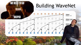

Andrej Karpathy: Tesla AI, Self-Driving, Optimus, Aliens, and AGI | Lex Fridman Podcast #333