Workshop: Advanced Vapor Sorption Techniques to Characterize Pharmaceutical and Porous materials

Okay, I think I will start now. Good morning everyone. My name is Nachal Subramanian and I would like to welcome you all for today's session on advanced vapor soption techniques to characterize pharmaceutical and porous materials. I'll be your host for today's session and I would like to thank you all again for taking the time to attend the workshop today. I hope it'll be interesting and it will be more interactive. That's the whole point. Because under normal circumstances, this workshop would have been conducted face to face, in an interactive manner at an university. And this time it was the University of Namur in Belgium. But due to the current situation, we have had to go virtual. And so we decided to open it up to people that are working in the Benelux region. So I would also like to give my special thanks to Professor Johan Uters at the University of Namur for helping me organize this workshop, for encouraging his colleagues contacts to attend. But unfortunately, fortunately he couldn't join us today. That's what he told me due to last minute appointments. But I have a few of his colleagues joining us. And I also have Nikolay Tomanov, one of the colleagues of Johan. And I think he would like to say something before we kick off the session. Nikolai, would you like to say a few words? Can you please unmute yourself and speak?

Yes. Sorry, I had a problem with the sound. Yeah. I would like to thank you for organizing this webinar. Well, unfortunately due to Covid situation, it's online, not a real seminar. So in next hours I hope that we will hear about DBS methods IGC for characterization of porous materials and pharmaceuticals. There are people with different applications for our application is probably more relevant. DVS for characterization of pharmaceutical compound and also some cultural heritage samples. But we will be happy to hear the rest of the presentation as well. Okay, I think it's time to continue.

Great.

Thank you, Nikolai. Thank you very much. Yes, I'm sure it will be interesting. There's a lot of DBS applications that Damiano has to show you. So I'm sure. And also at the end of the workshop, after all the presentations, we have a short DBS video to show the analysis and the operation of the software as well. I'm sure it will be very interesting. Now I think we'll just go to the actual program itself. And first of all, before that, let me just remind you all of you house rules just to say please remain muted during the presentations. Since it's virtual, it makes much more easier to avoid some background distractions and at the end of each presentation we will have some time for Q and A. But during the presentation if you have any questions, please feel free to type your question in the questions box in the right hand side. At your right hand side you'll see a questions box and please type it in there during the presentation and we will pick it up at the end of the presentation. And please do not hesitate to ask any type of questions. We want this to be as interactive as possible. And at the end of the session I will also send you copies of all the presentations from today. That is generally a very frequently asked question from attendees. Do we get copies?

Yes.

I will send you copies of all the presentations and you can also get in touch with me to run a few samples for demonstration analysis. Also free of charge. So we'll go to our first presenter. The first presentation will be given by Dr. Damiano Catano and his so just a little bit about Damiano. Damiano is our Senior instrumentation scientist and DVS product manager. He obtained his PhD from the University of St. Andrews in UK in 2015. His research project focused particularly on using porous materials for biomedical applications and then he joined SMS team in 2016. Since then he's been working on the development of advanced surface science techniques, particularly DVs using molecules as probes for studying various types of solid state materials. With that short introduction, I will pass it over to Damianu and invite him to start his presentation on dvs. All yours Damiano. Thank you.

Thank you very much. I'm gonna try to share my screen now so you can see my presentation. Okay.

Right.

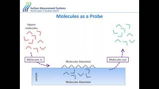
I hope you can hear me and I hope you can see the presentation on your screen. Yes. Right. So today I would like to talk with you about specifically dbs. This is going to be the overview of my presentation. I'm going to give you an introduction of the technique and the methodology that we use to collect data using dbs. And then I'm going to give you a few examples of application amorphous content calculation, phase transition. And in the last section I'm going to show you a couple of examples of application study using extra accessories, specifically camera and ram. So I'm going to start discussing how we perform experiments using a dbs. DBS is a gravimetric technique that analyzes the source capacity of sample by measuring the mass of the sample and the interaction between the sample and a gas phase solvent. In this case for example, we can use water for this specific type of experiment. So if we introduce water into the sample, the molecule will interact potentially in Two different ways. They will adsorb on the surface of the sample or they will absorb through the bulk of the sample. Now, whenever we reduce the concentration of molecules around the sample, they sample might release this molecule and the mass will progressively go down. So the process can be reversible. From a point of view of interaction, we can define these two phenomena as absorption and absorption as dependent from two different other process. So absorption is usually defined as chemisorption or physisorption. So a physisorption is a weak interaction. It's an interaction that is usually only happening on the surface and it doesn't require a lot of energy to happen because it's a weak interaction is usually a reversible process, which means that we can remove the molecule when we lower the partial pressure or relative humidity. Having said that, this type of interaction gives us a lot of information about the surface structure of the sample, specifically surface area, pore size and surface roughness or or heat of absorption and free energy. These are going to be more relevant information related to the presentation than my colleague are going to give you later. Specifically from the SCA point of view, for the free energy and also for the BET surface area, a chemistry is actually a more strong surface interaction. This is a covalent bonding. It can be reversible or irreversible. That depends on the energy involved in the process of interaction and the temperature in which you perform the experiment. But the main factor in this type of interaction is the fact that the sample is specifically designed to interact with the molecule of solvent that we are introducing. So in this case the process is specifically refined to interact with those molecules. So usually we are talking about catalyst dispersion, active surface area or acid base sites. Whenever the molecule are not only piled up on the surface of the sample, but also penetrate through the bulk of the sample. We have a phenomenon of absorption and absorption usually defines two phenomena, bulk absorption in which we have a phenomenon of diffusion. The molecule not only penetrate from the surface of the sample, but will have to diffuse throughout the bulk. And that changes specifically the kinetics of the sample solvent interaction, but also the time required for the sample to reach equilibrium. What we can analyze using this type of technique are phase transition, so vapor induced phase transition, so glass transition, recrystallization and deliquestant, which are phenomena that we are going to describe. In this specific presentation. We're going to also add information about total solution capacity and solubility parameter. We can get information and we can get information on DBS using diffusion and permeability as A phenomenon of absorption. Lastly, we have absorption into the lattice structure. And this is a specific structural change on the crystallographic point of view of the molecule that we analyze it or the sample that you're lining. So we start from some sample that iterates and it moves to hydrate or solvent, depending on if you're using water or an organic solvent. Now we can define the structure of the molecule that we end up and usually we can define it as stoichiometric or non stoichiometric. Stoichiometric is defined as definition that identify the hydrate of solvent in which we can count the number of molecules of the solvent that we are adding. So monohydrate or hexahydrate, non stoichiometric is in case we are not able to define the number of molecules that end up in the structure. The kinetic obviously can be studied using dbs and we can study the formation and the change in structure of this hydrate as well. So this is the type of information that we can get out of an analysis using dbs. And now I'm going to show you how we collect this type of data. So DBS technique starts from an older methodology that has been described in pharmacopeia 4 century that is called jar method. In a jar method you will have a series of desiccator that contains specific saturated solution of salts at the bottom of the desiccator. The saturated solution of a salt can generate a constant level of relative humidity. So each desiccator will represent a constant level of relative humidity at a constant temperature. So you can have lithium chloride, sodium chloride, potassium chloride, magnesium nitrate, and so on and so forth. And each one of them will have a different level of relative humidity. You can have 11%, 50%, 75% and so on and so forth. And what you would do is record an initial mass of the sample, load it in the desiccator, wait a couple of days, remove it from the desiccator, read the mass of the sample again, and move back and forth between the desiccator and the mass reading from a balance until you get a stable mass. Each desiccator represents a point of absorption in your isotherm. And that allows you to define the absorption capacity of that specific sample. Now, a DBS work basically in the same way, but is a continuous measurement. So we have a carrier gas that push molecule on the surface of the sample. And we also have a microbalance that constantly read the mass of the sample over time. So what we can do is load the sample create a method and collect data without ever interacting with the machine until the experiment is completed. So what's the difference between these two techniques? So in a jar method you require a significant amount of mass of sample. Higher is the mass and most repeatable is the sample. Specifically when you are running an experiment manually. So usually in a jar method you are, you're using grams of sample, while in a DBS we can use milligrams of sample. So the other difference is obviously the method that is used to define the way we reach equilibrium. In agile method, we use basically static diffusion of molecular gas on the surface of the sample. In a dvs, we have a constant carrier gas that pushes molecules on the surface of the sample. We usually use 200 milliliter per minute of nitrogen or 200 milliliters per minute of air. And that allows us to reach the equilibrium much faster. The last parameter we have to consider, apart from time, is cross contamination. Whenever we remove the sample from a jar, we expose it to a different level of temperature and a different level of relative humidity. Consequentially, we can change the equilibrium condition of the sample and we might have to recollect that point of data. Different people might do it at different timing. So that can change also the repeatability of the experiment. In a dbs, we load the sample, we record the mass going up and then down, and automatically we can collect the full data of absorption without ever interacting with the sample. And here I can show you an example of a difference in time required to collate the same set of data from from the same sample. On the left side we have the jar method, which requires about 300 days. And on the right side we have the kinetic data for a DDS, which for the same sample require 4.2 days. Moreover, if we take the data collected on the jar method, we can only increase the relative humidity. Consequentially, we can only measure the absorption of. While in a DDS, we can measure the full absorption and distortion and also measure the hysteresis, which is the gap between the measurement of absorption and desorption. So we can get a full study of the experimental data that we are collecting. So here is a schematic of one of our DDs and I'm going to guide you through the process of how we control the experimental generation. So, starting from the bottom right hand side, from here we technically have two reservoir. One is a dry reservoir, which is nitrogen or air, depending on what we are using for the experiment. And the other one contains the solvent that we're using, in this case, water. Each reservoir is connected to a valve that controls the ratio of the generation from the flow. So let's say we are running a dry stage. So we are, we want only nitrogen or air to push through the sample. So the valve that controls the wet side, so the water side is 100% closed, so 0% open and the dry side is 100% open. Let's say we are doing a step of generation at 20%. Then the wet side, the water side will be open 20% and the dry side will be open 80% for a total of 100. The two gases then meet in the plumbing and we record the reading of the relative humidity using a specific sensor. For water we use a humidity sensor. And then the gas line pushes the molecule into two separate chambers, a sample and a reference chamber, which are both connected to a microbalance at the top using handheld bio. Picture these microbalances, all pharmacies, two plated bugs in which we have a sample on one side and a reference on the other side. Sample and reference are perfectly identical, which means that whatever I put on the. The only difference between the sample and reference size is the presence of the sample itself. The reason is because we want to measure the water uptake mainly related to the amount of molecules that are absorbed on the sample itself. But we are doing it in a very simple way. We are just pushing molecules into the chamber and waiting to measure the absorption. Now we cannot control the molecules of water. Molecules of water will absorb not only on the sample, but also on the pan on the end and wire on the chamber itself. And we don't want to measure this data. We only want to measure the data related to the sample itself. So to do that we make the system symmetrical. So if everything that is on the left side is exactly on the right side, then the mass reading is not changing whenever we push molecular fluid. The only difference that we record is due to the presence of the sample itself. So that basically is the way we perform an experiment. The very simple procedure, if we picture a normal experiment of absorption and desertion, will have an initial drying stage in which we record the initial mass of the sample. And then we step up progressively the partial pressure or relative humidity. We measure the absorption and then we reduce the concentration of relative humidity and we measure the desorption. We wait for each stage for the sample to reach equilibrium. Then we record the mass of the equilibrium stage and then we can plot the percentage mass. Change the mass of the sample against the relative humidity to obtain the isotherm plot. So this is the schematic way we perform the experiment. And this is what the data will technically look like. So this is a plot of the kinetics data. So it has percentage mass change, which is the red line, target relativity, which is the blue line. And then on the x axis we have our kinetic data time. So this experiment is performed on a food sample and rice specifically. And here we measure absorption and desorption in two cycles. We have an initial drying stage and then we wait for the sample to reach equilibrium. At each stage we measure the full absorption and the full dissoption. So what type of information do we get from this initial plot? So as you can see from the data, the sample has a very, very high uptake of water, over 20% mass change. And it's perfectly reversible, which means that we can absorb and dissolve water in multiple cycles. And the mass of the sample always go back to the initial volume. So it means that the sample did not go through transition and did not change in the structure. Now if we take every equilibrium condition at each stage and we plot it against the relative humidity, we can get the isotope plot, which is right here. In red we have desorption, and in blue we have the desorption. So what type of information do we get from this data? Again, perfect reversibility of the sample, which means there is no change in the structure of the sample during the experiment. Very high uptake. But also there is a gap between the absorption and desorption. This highlights the fact there is a gap of hysteresis, which means that there is probably bulk absorption happening. Molecules have to migrate from the surface into the structure of the sample during the absorption stage. And then they have to migrate backwards during the desorption stage. Which means that during the desorption the molecule have to require more energy and more time to move out of the sample compared to the absorption stage. So if you look at 50%, for example, relative humidity, to get to the same level of mass during the desorption in the absorption stage, we have to go to a much lower level of relative humidity, which means that the molecule needs a much higher energy to move out rather than to move in. Now this experiment was performed at 25 degrees Celsius. And we know that kinetic are affected by temperature. So what I would imagine is that if we do the same experiment at higher temperature, we will close progressively this gas probiesteresis, because we are providing more energy for the molecule to migrate out of the sample. So this is my introduction to the technique now we are going to go and have a look at a few applications, starting from the amorphous content calculation. So to measure amorphous content, and I'm not going to define the concept of amorphous and crystalline, I think that's for a separate lecture, for a separate webinar. What I'm going to tell you today is how do we measure a percentage of amorphous over crystalline in a sample? So the way we actually look at amorphous to crystalline is to measure the transition phenomenon between the amorphous form and the crystalline form. What we are looking at, for example, is an experiment like this. So what you see here is very similar to what I show you as the application, as the introduction, an absorption and desorption of lactose starting from the amorphous phase in a dbs. This is pure simple water solution. So what we are looking at here is we start from a dry sample, which is amorphous, we increase the partial pressure and we measure the uptake. And what you can see here is that over a certain level of partial pressure, the mass drops. And after that stage, the mass proceeds to increase and then decrease. The interesting factor also in this data analysis is that the second section, the second section of this ocean does not present any phenomena of mass drop. So what is happening over here? So we start from a sample that is purely amorphous. And what we are doing is adding molecules to the sample itself. Obviously the molecule will absorb first on the surface, next to the bulk of the sample. Once they reach the bulk of the sample, what happens is that they cause a transition and they move from an amorphous phase to a crystalline phase. When you move from amorphous phase to a crystalline phase, the molecule reorder, which means that they have less space to actually be able to absorb water. Consequentially, they physically release water and they lose mass by consequences. So whenever you think of a sample, for example, of lactose, the amorphous phase of the lactose would definitely have a higher surface area. And Mission is going to talk about surface area later as a definition. But compared to the crystalline form of the same sample, the transition that you see here, the mass loss that you see here, is basically showing you what happened when we move from a sample that has a higher to a lower surface area by changing the structure of the sample. So if we look at the isotem plot, this is what you see over here. We have absorption, then a mass drop right here. And then the desorption stages changes completely. And in the second cycle we See that there is no transition left because there is no mass drop left. Now what we are going to do is try to quantify the difference in amorphous content between a sample and a series of other. So what we are doing here is we are going to define a sample as a reference, and then we are going to compare the value of amorphous content from that reference to every other sample that we are going to measure. The only thing that the DBS is not going to be able to do is to tell you the exact content of that reference that can be measured with other techniques like powder XRD or other organ techniques. The only thing we cannot do is define the reference. We have to pick a reference and then we are going to calculate the amorphous content compared to the reference. So how are we going to do this? We're going to isolate our first section of the data and we're going to focus on the mass drop specifically. So here is my mass uptake. The mass goes up and then we have a mass drop around 60%. If I split this data into two sections, and if I take, for example, 30% partial pressure, then in this case my material is fully amorphous. If I take 90% partial pressure, then my material is fully crystalline. So Those are my two factors. 30 is amorphous, 90 is crystalline. So I'm going to take a fresh batch of my reference material and I'm going to set up a second method that is exactly like this. I'm going to dry my sample and then record the mass change at 30%. And that is the mass I've taken amorphous. Then I'm going to drop the partial pressure and move up again to 90%. And here you can see my mass change going down because I'm moving from amorphous to crystalline. And then in the last stage, I'm going to go back to zero. And then I'm going to go back to 30%. And this is finally the uptake of 30% of the crystalline form of that sample. So, very simply, the delta between this value and this value is exactly related to the only dependent to the amorphous content. So I can measure the amorphous content of my reference material and then compare it to every single other material that I want to compare with the same structure. So what are the advantages of using this method before I move on to the next application? Obviously, this method is very repeatable and it doesn't require a calibration. Specifically, we don't have to create a calibration curve to Measure this amorphous content. We just have to define a reference material. There are two factors that we have to consider. We need a reference material that we have to find. And second, we, we need to find a solvent that causes our crystallization. We need to find a solvent that changes the structure of the sample from the amorphous to the crystalline phase. So what solvent should I use? More often than not, that material is being made amorphous using a solvent could be water from freeze drying or could be 2 solvent, a CO solvent and anti solvent from crystallization or from spray drying. So those solvents are the one that are going to test first to see if they can change back the amorphous to the crystalline form. Usually the solvent that is able to form the amorphous phase is also the one that is able to give you energy enough to move to the crystalline phase. So moving on to the second section of the application that I want to show you today is phase transition. Here is an example of the same type of material. This is amorphous lactose. And this type of experiment is not a step. We are not moving up the relative humidity step by step and measuring the mass up. What we are doing here is a different type of spec. This is a round. So what we do here, we start from a dry sample and then we step up the relative humidity in blue constantly at a constant speed. And what we are doing here is we measure the mass change, the red line in parallel to the percentage mass to the relative humidity increase. Okay, so if we think about a material that has no transition, a very stable material, let's say silica gel. If you picture the mass change of silica gel when you increase the relative humidity, what you would picture is the fact that you have a line for the blue line for the relative humidity, and a parallel line, a perfectly parallel line on the red line of the mass. The higher is the mass, the higher is the humidity, the higher is the mass, just in a parallel line. Every deviation from this parallel line means that the sample is going through transition, some sort of transition. Excuse me. So let's have a look at this data from the amorphous language. So what you see here is the fact that initially there is surface ocean, so more or less parallel line. Then we have a specific hump right here. This sump is usually identifying a glass transition phenomenon. What's happening is that the molecules stop piling up on the surface of the sample and they are trying to penetrate. But to do that, they have to move the surface of the sample from a Glassy form to a rubbery form. So this is what happening glass transition happen. Once the molecules are able to penetrate through the bulk, then we have bulk solution. Obviously, because the molecules are now able to penetrate through the bulk, the mass uptake has increased. Compared to the pure surface oxygen, there is more surface for the molecule to absorb. Now, we know that the sample is amorphous. So what happens is that at some point, the bulk absorption trigger a crystallization process. And we know that by this slide, before the process of crystallization causes a mass loss, so ards the mass loss of the sample caused by the recrystallization stage. So now, from these data that you see here, we can identify a point of glass transition. This is dependent obviously on the ramp speed of my method. But this tells us that this is a step of grass transition, and this is the relative humidity at which the grass transition happen at this specific temperature. Now, what can we understand from this data? Now, the main factor that we're looking at here is the fact that we need to define a ramp rate. So what happens if we do the same experiment at constant temperature, but we change the ramp rate? What we see is that by increasing the ramp rate, we increase the relative humidity at which the glass transition happens. So we go from 32% to about 42%. Now, we also can look at this line and project it to the Y axis and find a critical level of relative humidity, which is about 30%. That level of relative humidity is independent on the ramp rate, because the ramp rate there will be zero. So what we measure here is the tg. So the critical relative humidity at which the graph transition happen at a constant temperature, which is slightly different from what you get at dsc. DSC gives you a temperature. We give you a relative humidity at a constant temperature. Also, usually the value of relative of grass transition measurement on DBs compared to DSC are slightly lower because we are using a lot of solvent to move the glass transition to the next stage. So other phenomena of phase transition are obviously very simple drying curve. So this is a very, very basic experiment that you can do in DBs. You start from a dry sample, you bump up the relative humidity to 90%, you wait for the sample to reach equilibrium and then you drop it. And what you want to see is the mass drop. Can the material go back to the initial form and how quickly it goes back to the initial form? Now, this process obviously depends on the temperature that you do in the experiment. So this is, for example, 20 degrees Celsius. And we can do this experiment at different temperature and see how this affects the timing required for the sample to dry up. One of the important things to notice is that this is not really representative what a sample would see when we are running it in a normal condition. You wouldn't put a sample in 90% relative humidity overnight. All you would likely do is have a sample in a sealed container and expose it for a few seconds to a higher relative humidity, which is in your lab, and then close it again. And this is an example of what could happen in that type of situation. Here is a sample that is always at a lower relative humidity, but for a few minutes is exposed to a higher level of relative humidity. And here we have it at different temperature. Blue line is 25 degrees C, Red line is 35 degrees C. So what you see here is that the samples cycle up and then progressively down, but it never recovers back to the initial body. Now obviously the longer you expose it to high level of relative humidity and the higher will be the final water content, the sample itself. But one of the important factor is morphology change on the sample. So what happens when this cycle is repeated over and over? For example, I'm running this experiment from this batch, from this sample from my container from the last couple of months. So what you will see here is that every time we open and close the chamber or the container, we expose the level of relativity to high and low, high and low. And in the red line you see the mass change that goes progressively up and down, up and down, down, but it's cycling up. What effect this will have on the sample. Now if we have a look at the isocan plot of this set of experiments, you can see that we start from a lower mass water content and we end up with a very, very high water content. But also the morphology of the sample has changed. The sample has started from a free flowing powder and ended up with a cake material that is completely flocked and it doesn't flow anymore. So that changed the morphology and the physical properties of the sample. So this is something that we need to consider when we think about what happened in small burst of exposure or high level of humidity. So the last example that I have for you is accessory applications, specifically Cameron Raman. So how do we run in situ experiment with camera and ram? Here we have the DVS chamber, the sample chamber. Here we have a glass pan that we're using to run this experiment. So you will load the sample onto the span. And what you see is obviously that we're using a coarse span, which means that we can have a camera at the bottom of the chamber that collects photos of the sample throughout the experiment at the end of each stage of the experiment. So that allows us to collect data and see change in structure on morphology. We also have pistol shaped probe that comes on the top of the sample without touching the pan. And that allows us to correct Raman data at the end of each partial pressure stage. And this allows us to characterize the sample and see change in structure and potentially morphology of the sample. So what would the data look like? So here is a very simple example of Maltodextra collecting on camera. And here we increase the relative humidity to 95% from zero and we collect camera shot every certain amount of time. So at zero, at 30 minutes, at 50 minutes and you can see the sample going through clear deliquescent, moving from a powder to basically a puddle of water. It's very, very simple to perform this experiment. Now if we want to do it by following pure experiment, for example of glass transition and recrystallization. Just the data that I showed you so far here you can see an example sucrose. We start from a sample that is amorphous. We go through glass transition right here. Then we have a recrystallization stage. You can see the formation of the crystal and you can see how lower is the surface area of the sample compared to the two value and and then the pure deliquestion point at the end of the experiment. Now let's talk about Raman. What can Raman give us as information? Here is a very basic example of a DVS experiment on a food material. We start from 50% relative humidity. We do absorption and desorption in two cycles. And what we did is record the Raman data at the end of each stage. An easy things that we can do is overlap the data and see if there is any change, any transition in the spectrum that we are observing. So if we take the data collected in any condition in which we have altered so up to basically 1040%, what you can see here is that the plot of the Raman is perfectly overlapping. There is no change in structure, there is no evident change in the Raman data. However, if we look at the data at the end of the drying stage, specifically the Raman data, what you can see here is the fact that there are differences in the Raman peaks in the position of the peaks and the intensity of the peaks. Now this is particularly important for this customer that has this food production specifically because they can immediately understand if the sample is perfectly dry or not. By simply collecting a Raman spectrum and see where it ends in the Raman spectrum itself. A couple of seconds will tell you if the sample is perfectly dry or it has a small content of water. A more sophisticated example of application of Raman plus camera is a recrystallization study that we perform in collaboration with Institute of Technology in Germany for pan. Here is a crystallization process of catalyst. They provided the sample in a solution and they want to know what material they end up at the end of the crystallization state, specifically what polymorph of that catalyst we obtain. So we start from a solution of ethanol and what we do is we progressively dry the sample and we can follow the mass loss in DBS and with the camera. And you can see the random probe right at the top of the pans. Specifically right here, you will see the pans and you can see the camera collecting the data, but also you can see the Raman probe at the top. What we follow with the Raman is from the first point of view, obviously, the disappearing of ethanol. There is an abundance of ethanol in the solution. So we collected the spectrum of ethanol and what we can see here is the reduction of the concentration of ethanol in the sample pump progressively during the experiment. Now, that's very straightforward. We can obviously remove the background noise and we can get perfectly identical data of the ethanol compared to the literature value. Now, the most important part of the data was identify what type of polymorph. And if we get only one type of polymorph at the end of the crystallization stage, specifically, they identify the fact that there are four different polymorphs and they are identified by specific pith in the CN vibration between 2200 and 2300 centimeter to the minus 1. So we collected the data of the final product that we obtained at the end of the crystallization. And as you can see over here, we are able to identify the presence of one specific single peak, which is the one compared to the literature values. So this data allows us to understand that we get one single polymorph, not a mixture of polymorphs at the end of the process and is identifiable via ram. So the data collected here were run on ethanol, which is an organic solvent, and were collected using a specific type of sensor which we provide with our instrumentation, which we call speed of sound sensor, which measures time of flight to identify the concentration of unit organic solvent. We can provide these instrumentation specifically to run organic solvent experiment. The only thing that we provide is basically the sensor and a calibration for the carrier gas plus solvent combination, we have a series of solvent plus carrier gas that we provided up to 22 and you can get in contact with us and we can show you exactly what solvent we can use and how accurate we are to make measuring this specific solvent. Before concluding the presentation, I would like to highlight a couple of things that we perform here. So all the data that you have seen so far have been collected in this series of products. So DDS Adventure, Resolution and Endeavor. These three products identify a very similar type of incubator which allows us to control the temperature of the experiment and different performance from the point of view of accessory and solvent capacity. So DVS Adventure will allow you to run an experiment only in water. DVS Resolution will allow you to run experiment in water and or organic solvents. So single component and multi component experiment and DVS Endeavor can run experiment in water plus organic solvent, but it's a multi sampler system which means that you run five experiments at the same time rather than running one experiment each time. So with that I would like to conclude my presentation and would like to thank you for your attention and I would like to know if you have any further question in regard to my presentation.

Thank you Remiano. That was a fantastic presentation. And now we can open up for some questions. But I don't see any questions in the question box as of now. Please everyone feel free to type in your questions or you can also unmute yourself and ask your question. We will hold for some time and then we can. Yeah, we'll wait for some time for some questions. But maybe to start off, I have a question for you Damiano. How do you choose a particular solvent for a particular experiment, say phase transition or BET surface area. How do you choose a solvent?

So the choice of a solvent is mainly related to the potential interaction that the sample will have with my sample. So depending on what type of experiment I want to run, I will pick the specific solvent that I can use for that experiment. So in the amorphous content calculation that I showed you during the presentation, the choice of solvent will have to be the one that allows for a phase transition to happen. So a co solvent and an anti solvent that was used for the preparation of the sample itself. So for freeze dry would be water, for spray dry would be whatever acetone methanol combination that I usually use for this type of experiment. That would be my first choice. Now for VG surface series, slightly different, you want a solvent only interact with the surface of the sample consequentially. Well Mission is later. But really the solvent that you want are solvent that only have surface reduction. And in this case you want, you want solvent that basically have no condensation, but that are able to form a monolayer in the surface. So that depends not on the solvent itself, but interaction between the solvent and the sample. So you need to know a little bit of the chemistry of the sample and the surface of the sample itself.

Okay, thanks Damianu. Everyone, there is a poll question you can so please just, you know, select an answer and actually I have a question now from Timo Roloffs for Damiano. You mentioned that there is always a mass drop for crystallization, but some powders like lactose take up water to form lactose monohydrate. Do you then still see this drop in mass after crystallization?

So to answer that question depends on the composition of the sample itself and the content, the amorphous content. So when I'm working with a composition, what I'm measuring is not the uptake of every single component, but the sum of the total of the components. So if the material, for example, contain a lot of component form hydrates and that could have a massive mass uptake, that could cover a potential mass drop. However, if the amorphous content in the sample is high enough, then the mass drop will still be evident. For the formation of hydrate, usually they have a critical value of relative humidity that causes the transition. So it's usually anhedrous. Anhydrous. Anhydrous. And then over 50 or 80% it jumps to hydrogen. So it's a very distinct jump in the amorphous to crystalline formation is a mass drop on the other side and it usually happen at the lower stages depending on the amorphous content itself. Now if you're telling, if you're looking at a sample that has a 0.5% amorphous content and has the formation of a hydrate, then the hydrate will probably cover the mass straw because the mass trap itself is very, very small as a total. But if the ratio between the two is significant enough, you will be able to see both.

Thank you, Timo. I hope that answered your question. And we don't have any more questions. So I think you can always send us the questions by email if you, if you want later on. So, yeah, thank you. So I think we will. Thanks, Damiano. Once again, I think we will move on to our next presenter of the day. So the next talk.

Is.

The Next.

Presenter is Dr. Sabia Ahmed. John, are you changing the slide? So I have Dr. Sabia Ahmed here. Sabia is one of our application scientists for DVS and IGCSEA. She obtained her PhD in chemical engineering from Imperium College London. And after that she joined SMS as an application scientist and works on both SO option systems, DBS and igcsea. Now let me hand over to Sabia to give a nice talk on IGC technique. Sabia, over to you. Thank you.

Thank you, Nichelle for the introduction. I hope everyone can see my presentation and can hear me properly. So I'm going to be talking about igcsea. So this is the inverse gas chromatography surface energy analyzer. So I'm going to go through how the instrument works and a few applications that hopefully should be quite relevant to you all. So IGC was first developed in the 1950s. It uses gas phase probes to analyze a material. And in 2009, SMS Surface Measurement Systems has developed an IGCSE. This is a surface energy analyzer incorporated with the IGC. This is specifically designed to kind of determine the surface energy and the heterogeneity of your sample. But also because of these calculations you're also actually able to obtain other properties such as absorption isotherms, heat absorption, glass transition temperatures, solubility parameters and so on. So with regards to comparing the analytical technique with our IGC technique and analytical technique, effectively what it does, it uses gas vapor probes into a column and they separate out. And with this you obtain a few retention times based on the times that these probes leach out of the column. In inverse gas chromatography, it's quite different. We are actually packing the column of your own material and injecting some known probes that we know the properties of. Based on the interaction of these probes with your material, we obtain a peak based on retention time. And from this we can then analyze this peak and obtain different properties of the sample. So on the right hand side, this is what a typical IGCSE system looks like. It has two drawers on either end and a door in the middle. So when you open up each of these drawers, you'll have places for your vapor probes. This is your reservoirs here. So you have six on one side and six on the other side. And typically for surface energy measurements, we have a mixture of polar probes and non polar probes too. We can also measure humidity, so we can actually condition your sample to have a certain amount of relative humidity on your sample and then calculate and run our experiments based on that. And that will tell you how your sample actually properties change with relative Humidity and in this case, one of our reservoirs here would be water. The carrier gas we have throughout the system is either helium or nitrogen. And when you open the column oven, open this door here we have a column oven. So our columns go into either position one or position to, and it's surrounded by a column oven which can go to 20 degrees to about 150 degrees Celsius. Our detector is a flame ionization detector and this is very useful and very accurate in detecting organic probes. So as you can see at the bottom here, we have a few examples of what we can put into and measure in our system. As you can see, we've got quite a variety. So in these columns we have carbon fibre, cotton, hair granules, powder and so on. So effectively into a column we can try and measure it. And of course at the front, because we are using organic vapors, we have granite vapor leak detectors and our flame ionization detector runs on ignited by hydrogen. So of course we have hydrogen detectors there too. So this is a typical SCA column. And in comparison to our GC column, it is quite relatively easy to pack. So effectively what you start to do is insert some sun glass wall funnel in your sample of interest and plug in with some more silanised glass wall. And this just ensures that none of our material go into the IGCSEA system during the experiment. We have a range of different columns. We have 2 millimeter, 3, 4 and 10 millimeter columns. So our 2 millimeter columns for very kind of fine particulates, 3 and 4 millimeter column for kind of larger particulates. And the 4 millime column is for kind of like more fibers, fibrous material. Our 10 millimeter column accommodates quite large samples. So in case you have like a whole powder, a whole tablet or maybe a block of wood that you don't wish to actually break up, but you do wish to analyze a sample. We can put in a 10 millimeter sample. And because of the size, you do need a larger column oven to accommodate this. We also have a nice YouTube clip to kind of see how you prepare our samples that may be of interest to you. So before we begin our experiment, what we first do is pack our column with the sample of interest as seen here. So we're just funneling in some of our sample. We then select a few probes. So with regards to catching surface energy, we have a mixture of non polar probes which give rise to dispersive interactions and polar probes which give rise to more specific interactions. So we can choose which Probes that we wish to inject through our sample, we can use the concentrations we wish to inject them. So this is our infinite dilution or finite dilution as well. And then we start our experiment and based on the interaction between our probe molecule and our sample, we obtain different retention times which can then go ahead and analyze. So the system comes with two different softwares. We have a control software which is directly linked to the IGCSEA system. And this is where we set up all our experiments. And we can run about 10 different experiments sequentially. So one after the other. We also have an analysis software. So this is where we go ahead and analyze our raw data. And it's very simple. We effectively choose the beginning of the peak and the end of the peak and we calculate and what this does, it will fill in all these blanks here, which will be kind of peak area, retention time, peak max and so on and so forth. So we can then go ahead and analyze our data and this is automatic calculation. And we can also generate reports based on different analysis. And we can also have export the raw data as well if you do wish to kind of recalculate your own data. So there's a few different things you can measure using IZC sca. One of the most common ones are the surface energy. And because we're using polar components, we can also understand the acid base interactions of our samples. It's also possible to measure BT specific surface area, which Meesham will go through with you in the next presentation. We can also understand sorption, isotherms, permeability and solubility. We can also calculate work of adhesion or cohesion. And also, what's interesting, we can also have a heterogeneity map. So if we inject quite a few different concentrations of our vapor probe, we can actually understand and get a heterogeneity map across our surface, which is also quite interesting. So there's a few benefits of using igcse. The first is the two column position oven. So we can prepare two different samples and we can run them automatically and sequentially. There's no need for any outgassing facilities. So in the case where you may need to condition your sample just to ensure that there's no kind of absorbates that may actually influence your data in a different way. We, we also have this in situ conditioning where we dry our sample, we purge through some of our carrier gas and make sure that our sample is ready for the experiment. We have quite straightforward column packing procedure as I shared before. Sorry and also because we're using vapor paint, vapor phase, our injections are quite precise and accurate. We also have an automatic injection system compared to the traditional gc. And we have excellent reproducibility, especially for surface energy calculations. So before I showed you that our samples can go into columns. Alternatively, if you have a more planar sample, you can actually use this accessory which is called a film cell. So this film cell effectively sits beside the igcsea. So your sample will go in between here and we'll close our sample up. And these lines here, these connect where your columns would connect effectively inside the door and the position where your oven is. So these lines will fit here. So what we can do is we can measure the same experiments as you do. The only thing that we can't do is control the temperature. So because this is outside of the IGCSEA system, we don't have that temperature control. However, we do have the humidity control and everything else after that is the same. So what is surface energy? Surface energy is the most common technique used to measure measured property used by the igcsea. So this is analogous to the surface tension of the liquids. So we can understand the ability of the surface to react compared to the bulk. So to calculate the surface energy we need a couple of components. So we need the dispersive components. And this is in the form of your non polar probes. And these are in form of Alkanes. And this from this we can understand kind of physical long range interactions. We also have Lewis base components, this is our polar components, where we can understand our short range interactions. We need both of these probes to understand surface energy. So before we do a surface energy experiment, there's a few things that we need to know. First is our bet surface area, which again Mason will kind of go through how we can measure BT surface area using the igc. So this can be calculated using the IGCSEA or alternatively any other instrument. As long as we have this value here. We then need to know the molecular size of our probes. So the IGCSEA has a database with known with some probes and their properties. And if you did want to include some of your own, that's also possible too. So what the IGCSE does, we can kind of calculate the amount and moles that needed to actually obtain a certain coverage of our surface. And from that we start our experiment. And upon the interaction of our sample, we can calculate the retention volumes to determine surface energy. So there's a few other things we can understand with increasing surface energy because it's related to quite a few other properties. First is the wettability. So with increasing surface energy, we can understand the wettability of our sample. We will also understand the work of cohesion. So this is the likelihood of our samples interacting with itself and how kind of how cohesive they are with each other. We can also understand disorder and heterogeneity of our samples. So because we're going to introduce inject a few different concentrations of our probe molecule, we can actually understand any defects or porosity or anything on any kind of disorders on our sample. We can also calculate the work of adhesion. So say you want to understand the interaction between your sample and water. Let's say we can also calculate the work of adhesion between the two. So surface treatment is always quite interesting when we're understanding surface energy. So if you modify a sample in any way, we can increase or decrease the surface energy. And it's quite interesting to actually understand, understand this when actually treating your sample. So let's say if you're introducing a certain type of modification which would actually increase or decrease surface energy, we can actually understand what kind of modifications or different formulations that we can actually do. So for this example, it is I'm going to look at surface energy of D. Mannitol and its heterogeneity. So what's this showing here is we have crystallization of pharmaceuticals. So we have diamantitol and silence diamanitol. So we've carried out a surface energy experiment. So what we can see here is our dispersive surface energy. And what we can see on the x axis is our surface coverage. So we've injected at different surface coverages across our sample. So first of all, what we can see is a clear difference in the dispersive surface energy. So cyanide semantrol has a lower surface energy compared to our treated D Manitrol. What we can also see is a different kind of profile. So we can see a more linear profile with regards to the silonized D Manitol and a more curved profile with regards to D. Manitol. So what that's telling us here is that especially in this region, we are actually, when we inject these probes, we are actually accessing areas of the D Mannitol which contribute to heterogeneity. So this section here is quite interesting because we are injecting at infinite dilution, we can understand the heterogeneity of our sample. And the more curved our sample, the more heterogeneous our surface of our sample. So another way to understand our data is by taking our profile and integrating during a point by point integration, what we obtain is these peaks here. This is an alternative way to show, kind of understand your data. So what this is telling us here, the more broad our peak width, the more heterogeneous our surface of the sample. And the more narrower our peak width, the more homogeneous our sample. This is an alternative way of showing our data which is also quite interesting. So the next example I'm going to show you is an example to understand the surface energy of carbon fibers from Hexcel. So like I said before, we have conditioning in our system. So sometimes the conditioning can significantly affect the surface energy and the properties of our sample. So in this case we have sized carbon fibers versus the unsized. And we've also changed the pre treatment partition. So we pre treated one at 30 degrees and the other at 120 degrees. And from this we just want to understand what this kind of conditioning, how it affects our sample. So here like before, we have a dispersive surface energy on the Y axis and surface coverage on the X axis. And what we can firstly see is our size. Carbon fibers compared to onsized have a lower dispersive surface energy. And what we can also see is these profiles are much more linear. So again kind of suggesting that we have a more homogeneous surface in comparison with our unsights. So if we integrate under the curve, we obtain these peaks here. So we can see and understand that our pre treatment has a large effect on the unsized carbons. So if you looked at when we activate our carbon at 120 degrees with our pre treatment, we can actually see that we have a much more heterogeneous surface. So what's that telling us that 120 degrees we've activated sun sites on our carbon fibers. And this means that our probes can now kind of penetrate into these probes and kind of interact, interact with different higher energy sites. So this will give rise to a more heterogeneous surface. However, if we just carry out the experiment at 30 degrees, we, we will see that actually our probes don't actually reach any of those sites because they may be blocked. And this will give rise to more narrower peaks and therefore more homogeneous surface. So our next example is looking at pharmaceuticals. So what we're looking at here is we're looking at drugs, budesonide and salbutamol sulfate and our excipient alpha lactose monohydrate. And from this we just want to understand the uniformity and use IGCSE to understand kind of different properties of our material and to understand how the blending performance will work. And so we want to blend our excipient with our drugs. So what we can see here, we've calculated the dispersive surface energy. So this is our interaction with our non polar probes. And we can see that budesonide has a much higher surface energy compared to the other two. And using our surface energy calculations, we can actually calculate the work of cohesion. So this is kind of how likely our sample is to interact with itself. So what we see here in blue is our lactose and lactose interaction, budesonide budesonide interaction and our salbutamol sulfate. Salbutamol sulfate interactions. And in red we have our excipient interacting with our drugs. That's lactase, lactose budesonide and lactose subbutamyl sulfate. So let's just look at our budesonide and budesonide comparing to our lactose budesonide. So we can see that actually what is the, what this is telling us is that it has a higher work of cohesion and more likely to interact with itself than the lactose. So this is suggesting that there's a weak affinity between kind of the drug carrier. And this as a result could lead to a poor blending performance. However, if we look at the salbutamol sulfate compared to our lacto salbutamol sulfate, we can see there's our lacto salbutamol sulfate has a slightly higher work of cohesion. So it's more likely to interact with the subutinosulfate than the lactose than itself. So this kind of suggests a more stronger affinity between the drug and the carrier and as a result a much more better blending performance. We've also carried out some kind of complementary SEM images and what we can understand is the uniformity. So we can see that the salbutamol and our lactose has quite a better uniformity than our budesonide and our lactose, kind of reinforcing the fact that actually, yes, our subbutamol and lactose have a better blending performance. So my last case study is looking at solubilizer. So we're looking at drugs, carbamazepine excipient, which is soluplus, and we're comparing it to a reference excipient which is called codidone. So we want to understand will our carpamazepine actually, will our soloplus be a good solubilizer for our carpamazepine. So for this experiment we've carried out at 30 degrees, 10 milliliter per minute flow rate and no relative humidity. We've also carried out some solubility experiments and this was carried out at 60 degrees and injecting just kind of the one concentration. And these are the probes, non polar and polar probes that we use for the experiments. So what you can see here is our surface energy of each of our components. So carbamazepine solid and also our Solu plus with our carpamazepine and our reference solubilizer. So what we can understand from this is our we have the total surface energy, dispersive surface energy in blue and specific surface energy in. So what you can really see is our dispersive surface energy contributes more significantly to our total surface energy compared to the specific surface energy. What we can also understand is we can see that the carpamazepine has a high dispersive energy compared to the others. And this is due to the types of interactions and interaction with our probe molecules. We can also see our Solu plus and our extruded with our carbamazepine look quite similar. So they have quite similar properties which suggest that our carbamazepine has in fact blended well and dispersed into our Solu plus. So we can see that extrunatate with our carbamazepine looks similar to the solid plus than it does the original carpamazepine. This kind of gives us a suggestion that actually, yes, we have completely kind of dispersed our carpamazepine in our polymer matrix. We also calculate the free energy of desorption, which is the interaction of our sample with these four polar probes. So we have dichloromethane, acetonitrile, acetone and ethyl. So what we can understand here is first of all, we have quite significant differences in our carpomazepine, which is red and our soliplus. So these have quite differences in interaction with these probes. What's also interesting to see is our extrudate, which is in purple and as solid plus they behave quite similarly and interact with these probes quite similarly compared to just our carpamazepine. So again, this kind of suggests that the carpamazepine again has dispersed completely into the polymer matrix. What we can also understand is if we look at our reference collidon, it actually has quite different interactions with all our probes. So this is kind of suggests that actually surface chemistry of the collidon is actually very different from solublast even though they're both solubilizers, they may have different surface chemistries, which will actually kind of affect the way that they interact with the carpamazepine. We have then carried out the solubility experiment. So solubility experiment is very useful for excipients or drugs that are partially immoral, and for more crystalline material. Really, you should be quite cautious when interpreting these results. However, we calculated the results of the Solu plus and carbamazepine plus, our Solu plus and the collidon. So what we can actually see, understanding the solubility parameters, is that these two values are quite similar. So this means that again suggests that these two components would be more miscible with each other and can blend quite well. And this is supported by alternative data such as the DSC XRD and some SEM studies as well. So, just to summarise, the SCA IGCSE is very versatile and quite sensitive technique. We can analyze a variety of different properties, including solubility parameters, surface energy and some isotherms and heterogeneity, as we've seen in this presentation. And it's really a good way to kind of understand and compare different properties between samples, even subtle properties such as differences in surface chemistry, as we saw from our collidon reference experiment. So for everything that I've mentioned, we have some. A few publications with regards to everything that I've mentioned, also maybe a few case studies that might be interesting to you with regards to surface properties calculated by igcsea. So thank you for listening and if you have any questions, please do ask.

Thank you very much, Sabha. That was very, very nice and very clear presentation. I do have a few questions here. So the first one is what is a carrier gas for IGC experiments?

So the carrier gas we have is either. I can go back, it's either helium or nitrogen. So the carrier gas is effectively what kind of drives the system. And for this, in this case, we.

Have.

Yes, we have a helium or nitrogen going through our experiment. So this is really whatever you have in that's more accessible to you in the lab, because we've done some experiments comparing the carrier gas of nitrogen and helium and we've seen very little discrepancy. So there's no real difference when carrying out your experiments in either carrier gas.

Right, thank you. The next one is how do you condition precondition your samples before IGC experiments?

So for IGC sc, you would pack your column and insert it into the column position and before your experiment, or in Your experiment experimental method you would choose column conditioning. So effectively what that does, it introduces your dry carrier gas through your sample for a period of time. So you can choose whether you want to add certain temperatures so you can increase the conditioning temperature as well as the time, or you can just focus on just introducing just for a long period of time. And this will kind of ensure that kind of no absorption orbits are on your surface that may interact during your experiment. So effectively you'll have your conditioning step first and then your method.

Okay, there's one more question. So is the surface energy measured by IGC comparable with contact angle technique?

So yes, you can compare the two. The thing with contact angle is you're looking at specific kind of localized areas of your sample which can not necessarily give more realistic data because with the igcse you're looking at the whole surface of your sample. So you're looking at your surface chemistry across the surface of your sample. However, with contact angle you're looking at more localized places. And also it's very easier to compare the dispersive surface energy with contact angle and IGCSE because you're using non polar probes. However, if calculating specific surface energy, we're looking at polar probes.

So in order to compare the two.

Techniques, IGC and sca, you'd have to use the same polar probes for each. For each technique.

Great. Thank you Sabia. I don't see any more questions.

Thank you Nachal.

Thank you everybody for listening very much.

I think we will move on to our last presenter for today. Dr. Mei Shan. Goh Mason is our application engineer. She obtained her Master's Degree in Chemical engineering from Imperial College London, PhD where her research project focused on investigating the property properties of fragrance molecules with solid substrates by diffusion and sorption. She joined SMS in 2018 and since then she's been working on surface characterization of solid state materials using DVS and IGC techniques. So now she's going to give a presentation on BET surface area measurement using both DBS and IGC techniques. Over to you Meishan.

Thank you for the introduction and I'm sharing my screen now. I hope everyone can see it. Yes. Okay, that's great. So in my presentation I will just focus on the BET surface area determination using both of the technique we introduced previously, IGC and the dvs. And here's the outline of my presentation. So first we will have a brief introduction about the BET specific surface area discrimination theory, like different types of isotherm, the classical equation for BET calculation, and also different methods for The BET determination. And then we will go in detail for each of the technique with different case studies with lactose fibers as well as some freeze drying materials. So first from the classification there are six types of isotherms based on different soft mechanism. So the type Y isotherm here is very typical for some micropowers material having a relatively small so small external surface area, for example some active carbon, zeolites, silicas and those kind of material. For the type 1 isotherm, the limiting uptake is more dependent on the micropore volume rather than the internal surface area. The type 2 and type 4 isotherm are the normal forms of isotherm obtained with non powerless or macroporous material having the monolayer and multiple layer structure of the probe molecule. And those two types of isotherm are the one used for the BET surface area calculation where we use the monolayer region to calculate the BET surface area of the solid sample. The type 3 and type 5 isotherm represent some weak interaction between the probe molecule and the solid surface. For example, for most of the water isotherms obtained with the sample, it's really a type 3 isome like this one is more like some condensation on the surface that the absorbent interaction is much stronger compared to the interaction between the sorbet molecule like water molecule with the solid surface. And these kind of etherms are not suitable for the BET determination. And here's the classical equation from the BET theory where we have X is the partial pressure of the vapor above the surface, V is the amount of vapor absorbed on the surface. So if we take the left part as the ordinate and plotting against the X here it should be a straight line with the linear regression. So from the slope and the intercept of this line we can then calculate the vm, the monolayer volume and the sorption constant, the C value from the line and with the cross sectional area of the PRO molecule we are using from the literature, we can then calculate the BET surface area of the solid sample of inches. So it's very important to fit a linear line to calculate the BET model. To fit the model here, that's why we need to use the linear region from the type 2 and type 4 isotherm. And it's very important to get the monolayer region for the calculation where the probe molecule will interact with the surface forming the monolayer first and then interact with the first layer forming the multiple layers. But if there are too strong interaction between the PRO molecule, they will form some cluster on the surface Rather than cover the whole surface with the monolayer. And this will result in the type 3 and type 5 isotherm, like some condensation on the surface. And those are not suitable for the BET calculation. So it's very important to choose the right type of pro molecule of the interaction to get the right type of isotherm for the calculation. For example, here, with the example of a lactose sample with the less polar molecules, the shape of the isotherm is changing from the type 3 isotherm to the type 2 isotherm. So here's the water isotherm. This is not recommended to use for the calculation of bet surface area, but we will, if we are using like butanol, propanol or some methanol, ethanol, those kind of probe molecules, we will get, we will get a better result and also a better linear regression for the BET calculation. So we have different methods for the BET determination. The most common method like the volumetric method with nitrogen sorption, which is really good and reproducible for some porous material like silica zeolite or active carbon which has the surface area above maybe thousand square meter per gram. But this kind of technique has some limitation in terms of the low surface area material. For example, some fibers like hair fiber, carbon fiber or some pharmaceutical powder like the axin powder or some drug powder. In this case, the vapor absorption technique like DVS and IGC will give a more accurate and reproducible result for those low surface area materials. And also in terms of the experimental condition, the vapor sorption technique is using the organic vapors and applied at ambient temperature and pressure, which gives the surface area more close to the real world condition during the precising of performance. So with the volumetric method for the sample with the surface area around 1 square meter per gram, with nitrogen sorpting technique, it will give a relatively high relative standard deviation like 10% RSD which is probably due to the sample is absorbing a very small quantity of gas, which makes the relative error unacceptable. In this case we need to use krypton instead of nitrogen as the sorbet. But krypton is a quite expensive gas. And in terms of the experimental conditions for the volumetric method, it will be performed at some extreme conditions like the liquid nitrogen temperature or the very low pressure like vacuum drying. And these extreme conditions are not friendly to some sensitive or fragile material like the freeze drying material or some pharmaceutical material with the hydrogen water. So during the measurement at this, under these extreme conditions the sample will collapse, shrink or also change any Structures during the measurement, like losing some hydration water. So the mirrored surface area of those sample are not the original sample anymore. And it's not the surface area of interest during the precise performance. But in case of the vpersorption techniques, we don't have those kind of problems. For example, here with the inverse gas chromatography we will use the pulse injection of the single organic vapor at ambient temperature and the pressure. And we can measure as low as 0.1 square meter per gram of the sample. Still with a very high reproducibility like 1% relative standard deviation. And the common method, the common pro molecule we will use like the heptane, octane, cyclohexane or we can even use some ethanol for different types of materials. And it's also reported in this literature, in this paper about the effective surface area of the pharmaceutical ingredients. It's saying that the surface area of these low surface area material, the spray drying dispersions, are not accessible by the standard nitrogen sorption technique. Well, IGC method with the flow of gases at ambient temperature will reduce the risk of any structure changes within the sample during demarment. And then we will go in each technique individually. So the first one is dynamic wave absorption. As Damiano has already gave a really good introduction of the theoretical part in the previous presentation, so I'm not going in detail here. Just briefly, DBS is a gravimetric method to measure the mass change of the sample at different relative humidities. So if we take the change of mass when it's reaching equilibrium at different partial pressure and plotting against the relative humidity, we can then get the isotherm of desorption and desorption branches. And if we are using some organic vapors like octane or ethanol and Getting a type 2 isothermic for the BET calculation, we can then use the isoscelent from the DBS data to calculate the BET surface area of the sample. So here's the case study with the lactose monohydrate sample. And we did the octanesorption at 25° from 0 to 100% RH with 5% intervals. And here is the absorption isotherm of the octane sorption. It's a very typical type 2 isotherm and we have quite a lot of points between the BET range. So we only use the points between 0.05 to 0.35 to calculate the BET here. And with the BET equation in the previous slides, we can then convert this octane isotherm into the BET plot Here and from the slope and the intercept of this line we can calculate the BET surface area for this lactose sample is around 0.26 square meter per gram with a very good linear regression that's 0.999. And this value is quite consistent with the reported value in the literature for the pharmaceutical grade lactose sample. So here demonstrate the potential of DBS to measure the surface area of the low surface area material. And with the DDS technique we can also measure some very high surface area material like zeolite or silicas with the surface area above maybe hundreds or thousand square meter per gram. And the next technique is inverse gas chromatography. So the same here. Xavier has already given a really good introduction about the technique. I'm now going to in detail about the principle here. But if you are interested in the principle and if you have any questions, just contact us after the meeting and we can share you with some publications or the application notes and you can go in detail later. So here IPC as a gas chromatography technique has a really good reproducibility. And here we use the pharmaceutical powder, the paracetamol as an example. And we did 10 different runs on the same column here. And the result we get for this pharmaceutical powder is about 0.27 to 0.28 square meter per gram with the RSD around 2% which shows a really good reproducibility of the IGC measurement. And aggies technique also shows a good accuracy as well. So for example here with the BET standard, the CRM170 sample, the reported value for this standard sample is about 1.05 square meter per gram. And then we did the octane sorption with IGC technique at 30 degree with around 500 milligrams. And here's the octane isotherm. And this is the converted BT line also shows a really good linear regression here. And the reported value is 1.05. And the merit value of IGC technique is about 1.01. Just showing a good agreement with the literature value as well. And apart from the accuracy and reproducibility, another advantage of IGC technique is the system is equipped with the background humidity controller which allows us to add the humidity during the measurement so we can study the effect of the humidity on the surface properties. So for example here with the CRM171 sample at dry condition, the surface area of this sample is about 2.95 square meter gram. And then we add the humidity during the measurement. So with the Increasing of humidity at 90% RHT, the surface area of this sample drops over almost half of the original value which is probably due to the water molecule will compete the size on the surface and also blocking the available surface for the probe molecule. So in this case for this alumina sample, the surface area will increase will decrease with the increasing humidity. But in terms of the quotient it shows some different trends. So here's the quotient also with the humidity studies. So with the increasing of humidity in this time, the surface area of this coating sample is also increased by around 10% which is probably due to the hydrophilic character of the cotton fiber that the water molecule will go to the bulk and make the fiber swelling that increase the surface area with the increase in humidity. Another study example was the magnesium steel resample. So here also shows the increase, sorry the decreasing surface area with the increase in humidity here. But after you precondition at 110 degree here, the surface area at dry condition is around 6 square meter per gram. It's even larger than the original value we get at very beginning before the precondition which is probably due to the preconditioning process. Just remove any maybe tightly bond water or some hydration water in the structure, changing the structure during the measurement. So the surface area is even larger than the original value. So if we mirror this kind of sample directly with the nitrogen sorption technique at liquid nitrogen temperature during the measurement, the hydration voltage will be lost. And this probably be the value we will get from the volumetric method. But it's not the original sample of interest anymore. And it's not the real surface area during the precising of performance. And in case of the volumetric, in case of the vapor sorption technique, we can detect this kind of difference before and after dehydration water losses. So the case study here for IGC technique we measure different fibers, we measure the surface area of different kinds of fiber and the material we have here. For example, we have one synthesized cellulose fiber, the bell meat sample. And we also have two nitrobex fiber, the kidnapped sample and the flex sample. And here's the macroscope images of the 3 fiber sample. So as we see the biomead sample and kidnapped sample, the surface of those two fibers are quite neat and clean. And it's very uniform, it looks like very uniform. But in case of the flex fiber here, it shows some kind of fragments of cuticles on the surface. And the surface is not as smooth as the the other Two samples. And then we did the IGC measurement to measure the BT subseria of all three fibers for each column we were repeated for three times and here is the average value for the three different runs. So the standard deviation for all the sample is below 5% relative standard deviation which is quite good reproducibility for the IGC result for different experiment to experiment measurement and the surface area for the first two samples, the Bell meat sample and Kinect sample is about 0.5 square meter per gram. While for the flex fiber the surface area is almost three times larger or three times as large as the other two sample about 1.4 square meter gram. And this high surface area of the flex fiber is related to the surface roughness as shown in the previous microscope images. So here demonstrate the dbs. Oh sorry. The IGC measurement for the surface area determination is related to the surface roughness of the solid sample. And this is the result within only one column. The same column we repeated for three times and then we pack different columns and measure the surface area for different batches. And here shows that the two best fiber, the Flex fiber and Kinect fiber has much higher dash to batch variation compared to the Bell Mead fiber, the cellulose synthesized fiber. And this is expected as the nitrofiber as irregular structures on the surface and also shows some heterogeneous properties as a natural fiber. But for the synthesized fiber it will be more uniform and more homogeneous in the nature and that will result in the less batch batch variation. So as the IGC has a very good reproducibility, it also has the potential to mirror the batch to batch variation of different kinds of fiber or the powder sample still with a very good accuracy. And this is the publication reported by the Dr. Lagrasse and Dr. Conda and this is a reference paper. So if you're interested you can have a look later after the meeting in detail. And the last case study I have here is from spell group at Imperial College about the free strabol. So both nitrogen sorption technique and IGC method was used to determine the surface area of these freeze dry biological materials. So for nitrogen methods it was degassing at 30 degree and vacuum overnight and the experiment was done at liquid nitrogen temperature and in case of inverse gas chromatography it was preconditioned under the flow of helium for two hours at 30° and the experiment was done at 20° with the Octisor option. So here's the result. It's also the same columns repeating for three times. So The VT surface area for this kind of sample is below maybe around 1 square meter per gram or even less than 1 square meter per gram. And the relative standard deviation for the IGC method is below 5% RSD and it's much lesser than the standard nitrogen sorption technique. And this high value of the RSD value of the nitrogen absorption technique is probably due to the larger depth volume of the instrument during the measurement which becomes critical for those low surface area material. And here's a summary of the two methods Nitrogen method and IGC method so the advantage of IGC method in this case is we can determine the surface area with very low surface area materials still with a very high reproducibility and it also has the potential to add the humidity during the measurement to so we can study the humidity effect on the stability of this kind of freeze drying material. And this is a reference paper for your interest. Sorry. So just to summarize my presentation, DBS and IDC are two vapor sorption techniques used for the characterization of different solid sample like pharmaceutical powder, the fiber sample or the film sample. And then measuring the isotrim of the organic vapors we can determine the surface area of different solid sample especially for some low surface area material with very high reproducibility and accuracy. So I hope you will find DBs and IGC useful in your future stories and thank you very much for your listening. Please let me know if you have any questions. Thank you. Thank you very much.

That was a fantastic presentation and it's very good to know that the BET values obtained by DVS and IGC are comparable to the standard volumetric technique which requires vacuum, very low temperatures, etc. So it's good to know that have a question from Eva. If you have a DVS equipment that only uses water, can you still use it for these calculations?

Yes. Thank you for your question. So as I mentioned the most important part is we need to obtain a type 2 or type 4 isotherm for the bet calculation to fit the linear line. So if you are using water and getting a type 2 or type 4 isotherm then you can use water as the pro molecule to calculate the BT surface area. But in most of cases water will make the condensation on the surface and this will result in a type 3 or type 4.5isotherm. So it's not suitable for the bet calculation. So it's all depending on different method, different samples and different isotherms. I hope this answer your question.

Thank you Mason, there's another question From Veronique. Matthew, have you made any case study with polymers?

Yes, of course we have the case studies for both of the techniques with polygon polymers like for determining the surface area or surface energy or even the glass transition temperature humidities. So if we're interested we can contact you later and share you with some application notes and publications.

Thank you for any more questions while answering the question on the screen. Another question while we're waiting. So what is the difference between these two sorption techniques for measuring bet one preferred over the other for certain type of samples?

Well, both of the techniques are suitable for different kinds of samples like powder or polymer. But the difference is DBS is very suitable to control the high humidity sample. Sorry, the high humidity. And we can go like 98% relative standard deviation. So we can measure the porous material like zeolite or silica. But as you see in case of the system limitation is doing the post injection of single organic vapor. So we cannot measure the surface area for the sample. Maybe about 150 square meter per gram. It's more accurate to control the infinite dilution. And yeah, I think that's the most significant difference between the two different techniques.

Okay, thank you very much Mason. That's all the questions we have. Thank you again. So now we are almost end of the session today we just have one more thing to show you. We will be showing a short video on the DVS analysis and software demonstration. A very short video. If in case you don't hear the sound from the video, please remove your headphones if you're using them because for Some reason the GoToWebinar platform plays audio only out of the PC speaker directly. So yeah, so I think John, if you can play the video.

Great.

Hello, My name is Dr. Sabia Ahmed. I'm an application scientist here at Cervus Measurement Systems. And in this video I'll be showing you how to plot isotherm data and kinetic data using the DBS software. So prior to analysis I'm going to show you a typical water absorption method that has been carried out to analyze the data.

This is the typical DVS control software.

And I'm just going to quickly show how to load a method. So we start from method and edit method and choose one of the files that you want to edit. And here it shows a relative humidity experiment starting at 0% RH and increasing by 10% steps to 90% RH. You can measure the stages in terms of time here or dmdt. For this experiment we've measured absorption with regards to DMDT where DMDT is 0.002 and this ensures the sample mass reaches equilibrium of a difference between 0.002%. Before moving on to the next stage, you can also set the temperature for the experiment and you can also select which position your solvent is in. For this experiment, our solvent is water and it's placed in solvent A. So after the experiment is completed the software generates a DAT file and this needs to be converted into an Excel file. So if you go to Excel and click on Add Ins and the first tab and DVS Plot manager and we can import our DBS data. This is the so you can locate the DAT file and open it here. Alternatively, if you've already created the Excel file, you can click Open Data Files and locate the data file from there. So here we have some options on how to plot kinetic data. On the right hand side there are a number of different parameters to choose from to plot our data using the x axis, y1 axis and y2 axis. On the left hand side there are some tabs for shortcuts which are frequently.

Used to generate plots.

The first one is the relative humidity plot. Here it's possible to compare the target relative humidity set by the control software and the measured rh which is the relative humidity during the experiment. Ideally these two should be both in and with very little discrepancies. Next we have the temperature plot. This shows the temperature stability during the experiment and as you can see here, the temperature is stable at 25 degrees. Next we have the drying curve. If we have a sample with unknown moisture behavior, it's useful to set up a drying step at the beginning of your experiment and here it's possible to view it separately and see how much mass of the sample has been lost during the experiment over time. Next we have a mass and RH plot. So here we have three experiment time on the x axis and mass and target rhythm on either one of the y axes. This plot compares the RH to the target RH to the actual mass of the sample during the experiment. So as you can see here, the sample has a slight increase of mass.

At each state of RH until it.

Reaches about 19 milligrams and during the desorption the sample loses some mass at each RH state. So it's useful to plot the actual mass of the sample sample during the experiment. The next plot is the DMREF and RH plot. This plot shows the change in mass of the sample compared to the reference which is shown in red and the target relative humidity shown in blue. It's important to note that here the default setting for this plot is set to auto detect mass. This takes the end of the mass of the drying stage at its initial M0. However, depending on the experiment, this isn't always suitable. So for example, for experiments which don't start at 0% RH, it's more appropriate to click this option here and to recalculate the data. Also, it's possible to generate custom plots. For example, if you want to plot a graph for solvation ratio, you keep time as the x axis and select solvation ratio. This plot is necessary to input the adsorbate molecular weight. So if you have water, this would be 18 and also input the sample molecular weight. So in this case 65. And then we can click Custom plot. This generates a plot for the solvation ratio which represents the molar ratio of the sorbed vapour onto the sample mass. So all the plots that I've shown here are examples of plots for kinetic data. The other option is to analyze isotherm data. So we go to add ins and click the second macro which is the DBS isotherm analysis. So here, like previously, we have two tabs which is import data and open data pile and these other tabs going through. How to plot the isotherm Isotherm is calculated based on the sample's equilibrium uptake at each partial pressure step. So prior to calculation we need to input a number for the isotherm average points. So here it's five. We can go ahead and press calculate isotherm and a table is generated of the isotherm data for desorption and adsorption. We can then go ahead and click plot isotherm. So it will use the data generated from the table to plot adsorption and desorption plot and in between is the hysteresis. You can also go ahead and plot hysteresis. So this is the difference between desorption and desorption isotherm. So looking at the isotherm we can see that there is narrow regions at the end and at the beginning of our isotherm plot. And this can be viewed in our hysteresis plot where both extremes show relatively low isotherm hysteresis percentage. So here we have some isotherm plot.

Options on the right.

So we can also customize the plots. So if the DBS has carried out multiple cycles and it's possible to select which cycles to plot. Also, if in the experimental data some data points are missing the software can ignore these blank cells and similarly during an experiment if we have blank half cells we can also ignore these cycles. So typically an isotherm is plotted with a curved line. However we can also plot as a straight line isotherm and this is sometimes useful to see a hysteresis a bit more clearly. So here we have our curve plot and here we can see slight difference in a straight line isotherm plot. Finally, there is also an option to add isotherm with regards to the solvation ratio and for clarification it is useful to remove the mass chain from this plot. We can then go ahead and plot our isotherm. This generates adsorption and desorption isotherm plot with regards to solvation ratio.

Thank you.

For watching the video. I hope you been useful and if you have any further questions with regards to plotting your data, we require any information with regards to software, please visit our website@servicemeasurementsystems.com or alternatively email the science team@scienceervicemeasurementsystems.Com.

Okay, so thank you everyone for attending the workshop. I hope it was useful and gave you some insights into how these techniques option techniques might help you in your research. As I said before, I can send you copies of these presentations and you can go have a look. Let us know if you have any questions. Also, we'll be happy to hear from you if you're interested in sending a couple of samples for demo analysis. Thanks. Thank you Ann. So yeah, so that's all for today. Bye now and stay safe. Thank you everyone.

Sam.