Workshop: Characterization of polymeric materials by vapor sorption techniques
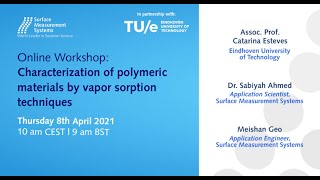
Surface Measurement Systems demonstrates Dynamic Vapor Sorption techniques for analyzing how polymers and porous materials absorb and adsorb gases. The workshop covers DVS principles, experimental modes like step and ramp testing, and real applications including VOC capture and SO2 sorption on metal-organic frameworks.
Questions this video answers
February 10, 2022
Approximately 1 mg to 10 mg (depends on expected uptake).
Mass changes down to ~0.1 micrograms can be measured.
Typical flow DVS (Resolution/Endeavour) operation: about 5°C to 85°C; some instruments/supporting options cited 15–50°C for certain solvent calibrations under air, and preheater up to 200°C.
Vacuum down to ~10^-6 torr; capable of gas sorption up to 1 bar in vacuum mode experiments.
Chapters
Good morning everyone. I hope you can all hear me. My name is Nachal Subramanian and I will be your host for today's workshop session. First of all, I would like to welcome you all for our workshop on characterization of polymeric materials using vaporsorption techniques. So today we'll be covering a technique called dynamic vapor soption DVs. And I would like to first thank you all for making it today to the workshop a little introduction to Surface Measurement Systems as a company. So we are a UK based company, we are the world leaders in option science and the company has been around for more than 30 years now. SMS develops and engineers innovative experimental techniques and instrumentation for physicochemical characterization of complex solids. We specialize in mainly two techniques, dynamic vapor sorption and inverse gas chromatography. Today in this workshop you're going to learn all about the DVS technology for polymer characterization. And this workshop is a collaborative effort between Surface Measurement Systems and Eindhoven University of Technology in the Netherlands. Associate Professor Katrina Esteeves at Eindhoven University has been really very helpful and supportive in organizing this workshop today. She is one of. She's our guest speaker for today. I'm very pleased to have her as our guest speaker. I would like to give my special thanks to Katrina for her support. She kindly accepted my request to be our guest speaker as well. You will see on our agenda, one of the talks is going to be by Katrina later on today. So with that I think I should move into the actual program. So we have our agenda on the screen now. So the first two presentations are going to be DVS presentations by Surface Measurement Systems by my colleagues here. And the third one is going to be a talk by Katrina Esteeves at Heindhoban University talking about the role of DDS in their research group and examples of materials that she analyzes using dbs. It's always very nice to hear from our customers, so I'm really looking forward to that talk. And in the end we're going to have a little demo of the instrument software and the control and analysis software. So before we go into the session, I just would like to all remind you all a few house rules. Since this is a virtual workshop, I'm sure you've been used to this kind of an environment for the last year or so, but I would just like to remind you that you'll all be muted during the presentations just to avoid some background noise. And at the end of each presentation we'll have some time for Q and A during which you can raise Your hand, you can use one of the buttons on the right which shows a hand button. You can click that and we will unmute you and you can ask a question yourself. Or, or you could also type in your questions in the questions panel during the presentations, anytime during the presentation and we'll pick that up for the speaker to answer at the end of the presentation and at the end of this today's workshop I will also be sending you copies of the presentations from today. So you will have and this is also recorded. So if you want a recording please feel free I can send you the link. So with that I would like to move on to our first presentation for today. The title is Introduction and Basic Applications of DVS by Dr. Sabia Ahmed. Sabia is one of our application scientists for DVS and IGCSEA. She obtained her PhD in chemical engineering from Imperial College London and then she joined SMS as an application scientist and works on both option systems DVS and igc. With that short introduction, I will now pass it over to Sabia for her presentation on dvs.
Thank you Nachal. I'm just going to share my screen, so thank you for joining the workshop. My first presentation is going to look at the introduction to the dvs, how it looks like, how it works and a few applications as well. Just to outline the presentation today I'm just going to go through what the dynamic vapor absorption system is, how it works as a gravimetric absorption instrument and a few applications and examples. There's a few different ways to characterise solids. We can first use energy as a probe molecule and this is in regard to spectroscopy where we can use light and x rays and this is to obtain analytical and structural information. You can also similarly use heat as a probe where we can get information such as calorimetry and more thermodynamic information. However, in the DBS we're actually using molecules as a probe and this is looking at the sorption techniques and so we can understand more thermodynamic, chemical and structural information of your material. So when we're using molecules as a probe, what happens in the DVS system is we inject our or introduce our vapor molecules onto the surface of our sample and depending on the interaction between the sample and the molecules absorbed, the molecules can either be adsorbed on the surface of the sample or be transferred into the bulk of the sample. The molecules can be absorbed into the bulk of the sample. This is adsorption process. We also have a desorption process where the molecules are released out from the sample. So there's two ways molecules can interact with they can either adsorb and in this case we're looking at more physisorption and chemisorption, or they can absorb into the bulk and into the lattice structure of the sample. So if we're looking at the adsorption, we're looking at more weak interactions. The PRO molecules may not necessarily chemically bind to the surface. And in this case we're looking at more reversible sorption. This kind of property we can understand kind of structural properties of the sample. So looking at surface area and porosity, we can also understand more chemical interactions such as surface sorption capacity, surface energy and heterogeneity. We can also understand heat absorption free energy of the samples too. With regards to chemisorption we're looking at more stronger interactions. So this is where PRO molecules may actually covalently bind to the surface of the sample. This can either be reversible or irreversible depending on the strength of the chemisorption. And this is quite interesting because we can obtain different other properties such as titrate, acid base sites, active surface areas and catalyst dispersion. So when molecules interact and go into the bulk of the material, we're actually looking at absorption. So we're able to penetrate into the lattice. And for this it can be either reversible or irreversible. And in this case because we're looking at bulk interactions, we can understand kind of structural properties such as vapor induced phase changes. This is for example blast transition crystallization or deliquescence. We can also understand chemical properties such as total absorption and solubility parameters and also kinetics such as diffusion coefficients and drying kinetics. We can also understand absorption into when we're looking at absorption to the lattice, we can understand solvate formation. This again can be reversible or irreversible. So we're looking at kind of looking at hydrate and solvate channels and understanding the kinetics. So we can actually compare this method to a static method. The static method here is the jar method and this can be comparable to our dynamic wave absorption. And for the jar method we need various different jars for each level of relative humidity. So in the static sorption method we introduce the probe molecules, but we have very slow achievement of equilibrium. This is because it's only depending on Brownian motion of the molecules being transported. However, in our case we're looking at fast equilibrium and more optimized flow rates. And in this case we can actually have More control over over the species onto our material. And this fast equilibrium of course speeds time of your experiment. So whereas in the jar method we can take a couple weeks or even months with a single data point, with the dynamic vapor sorption method we can take less than a whole day for a whole experiment, the jar method we need quite a lot of sample. So we need from 1 gram to tens of grams of sample. However, because in our system we have quite a sensitive balance, we only need about one to ten milligrams of our sample. The jar method typically relies on taking out and removing the sample from the desiccator and weighing it every time. And this of course can lead to risk of contamination and experimental error. However, in the DBS because we're weighing the sample constantly throughout the experiment, there's no contamination or loss of sample. Also the drum method, the only thing we can really obtain is a sorption curve and we can't really obtain the desorption curve and look at any hysteresis involved within the dbs we can measure sorption and desorption and so we have more information about our sample, especially in regards to kinetics and morphology changes by looking at the hysteresis gap. So GBS is a gravimetric technique. It's constantly weighing your sample over a period of time. By changing and looking at the changes in relative humidity we have an ultra sensitive balance which means that we can use a lot less sample and we can use real world conditions so we can run the experiments how it's more representative to how you use a sample. So in this case we can preheat the sample, we can do at different temperatures and also we have a wide range of vapours. We can use water and organic vapours. So this here is showing the family of our DBS products. So at the top here is our DBS Intrinsic plus. It's our smallest instrument and can only do water vapor sorption from 20 degrees to 40 degrees. It's really useful if you're only just using water for your experiments and it doesn't take much space up in the lab as well. We also have devious adventure and this is surrounded inside an incubator. So this again is water only, but temperatures can go from 5 degrees to 85 degrees. And we also have camera and Raman options and preheater options as well. The DBS resolution can use water and organic vapours as probes. Again from 5 degrees to 85 degrees to a very good temperature stability. Just like the adventure and again, we can use camera Raman preheater. And in this case, because we're using organic vapors, we also have a speed of sound sensor configurated in the system DBS Endeavour. Again, water and organic vapor gases. And this time we actually have five chambers here. So in this case we can actually measure five different samples in one go. So this is really useful if you have some samples that you wish to run in one method all at the same time. We also have a TVS vacuum and in this case we can present our sample under vacuum conditions. And again, we're using water and organic vapours and we're able to in this case preheat the sample up to 400 degrees, whereas the other instruments we can preheat from 200 degrees. So this is looking at the DVS resolution. So this is what the system looks like. So this is going to be placed inside an incubator for temperature control. We have the solvents here, another solvent bottle behind here, so we can do two different solvents. We also have a reference sample and your sample pan. And your reference pan.
Yeah.
And the balance is underneath this hood. So this is the schematic of the DVS resolution. So in this case I mentioned, the DVS resolution can actually use organic vapour probes as well as water molecules. So we have a tonic probe and the speed of sound sensor that we mentioned. And these go through the mass flow controllers. And in this case we have air or dry air or nitrogen as our carrier gases. So here is our reference pan and our sample pan. So these will be identical pans and you would only apply a sample and place your sample in the sample pan section. This is held all together by a micro balance which is constantly weighing the sample during your experiment. So our balance is very sensitive and very, very accurate. So we can measure mass changes of up to 0.1 micrograms and have very little noise as well. So like I mentioned, if you can do organic vapor and water as our probe molecules, we can do competitive absorption of two vapours. The temperature went from 5 degrees to 85 degrees and very good temperature stability. So this is showing you one of our panels on the DBS system. And what this is showing is the mass uptake time and what we can see is actually long term kind of temperature stability. This is looking at 25 degrees. And we can see we have very little variation in mass over time. We're also able to offer a preheater which allows a sample to dry prior to any experiments for up to 200 degrees. We also have a wide range of different humidity levels. So we can go from 0 to 98% relative humidity. And this panel here is showing you the. This graph here is showing you the humidity stability. So what we have here is our steps of humidity in green and red. So target versus actual, you can see they're in very good agreement with each other. The blue line is increasing the sample temperature. So what we can see, even though we increase the sample temperature from about 25 to 50 degrees, we still gain very good agreement with our actual and target partial pressures of our systems. We are also able to carry out true zero drying at 0% relative humidity. So what this means is that we're actually able to dry our samples completely at 0% humidity. And this is something that's comparable to our competitors, which, as you can see here from the example of naloxone, we can see that with our competitors, we don't necessarily reach 0% and complete dryness for our samples. However, in our system, we are able to reach true zero relative humidity and completely dry our sample prior to any experiment. So this ensures that whatever we obtain from our experiments is purely from our sample. We also have a speed of sound sensor. So in this case, this is placed at the back of our system. And this is a very accurate device to kind of measure the concentration of our organic vapor probes at different temperatures and different relative humidities. And this is in place of the dew point analyzer, which is used before. And this gives a much more accurate measured reading. We also have different calibrations, so different solvent calibrations. We have our speed of sound sensors. And these probe monitors that you can see here are all calibrated onto the system and at different temperatures as well. So at different temperatures, you need to kind of recalibrate the solvents. And so we have these solvents that can be used from 15 degrees to 50 degrees under air, and these can be used under 50 degrees nitrogen. And the gases below are typically for the vacuum system and from 10 degrees to 50 degrees. So there's a few accessories that we have with our system as well. We have a camera option. So this goes underneath your sample pan area. So the camera would be placed under here. Your preheater can also be placed here. But in this case, we can't use the preheater and the camera simultaneously as they go in the same position. So the preheater, sorry, the camera will go under here. And this will take a picture of your sample during the experiment. So in this case, what you would have is a picture taken after Each relative humidity step. In this case, we can actually develop a video of your sample as the experiment is going on. We also have a Raman option. In this case, we're actually looking down at our sample from this angle here. So this area here is now free. So now you can actually put in your preheater should you want to, or your camera. So we have an option for Raman, and this is quite interesting because you can actually obtain Raman spectra at each. At the end of each level of relative humidity. So we can take it at the first end of the 0% step and then the steps in between and the last steps. So we can actually see how the sample is changing with regards to kind of different functional groups on the sample and we can compare them different relative humidities. So this, this example, we're looking at the DVS with Raman and looking at the amorphous lactose changes at 25 degrees. So this is the typical DVS data that we've obtained. So we've introduced different. Excuse me, we've introduced a drying stage here and introduced different levels of relative humidity for our sample over time. And we've actually done two cycles. So this bit here is our adsorption and desorption. So that's cycle one. And again sorption and desorption cycle two. And our red line is actually the change of our sample mass in reference to the changes of relative humidity. So what we can see here first is we're first drying the sample 0% RH and then increasing the relative humidity in the system. And this leads to an uptake of the probe molecule here. What we can see at this place, around 60% relative humidity, we're actually getting a change in our sample. And this is going from an amorphous state to a crystalline state. And in this case, because of the change of our sample going from crystalline to a crystalline state, what we're seeing is that we have more of a lattice structure being formed. And since the lattice structure is quite tightly packed, we're actually losing this mass uptake. That's why we see a drastic drop in the uptake of mass. And this change is quite constant with increasing relative humidity here. So we can see that there's definitely a change from an amorphous true crystalline state. And looking at the second cycle is useful to kind of immediately do a second cycle, because what we can see is actually this phase change is irreversible and very different from what we obtained from the first cycle. We can see that this change is a permanent change from a norm to a crystalline state. We've also coupled it with a Raman data. So in this case we're actually comparing 0%, 40, 60 and 95%. And what we can see at the lower percentage Rh in our amorphous state, we can see that we have a particularly different Raman spectra compared to our crystalline state here. So we have the intensity is much more greater. We have a few peaks that were not there before and are there now. So we can actually monitor the change using Raman. And again, we've also coupled this with a camera and some video images, so we can see the difference of our sample in the amorphous state compared to our crystalline state. So like I showed before, we can actually have two cycle step method for our DVS experiments. So in this example we're looking at the moisture kinetics and moisture absorption of rice starch. So in this case we have our experimental target, relative humidity in different steps up until about 90% relative humidity. So absorption and desorption. And we've also included a second cycle, again absorption and desorption. And our red line is our mass uptake of our rice starch material. And what's interesting in this case, actually we are getting the same experimental data for cycle one and cycle two. So in this case we can see that it's a reversible experiment. So yeah, just to clarify, this cycle one and second cycle, and this at the beginning is our drying stage. We can also plot an isotherm. So at the end of each step here we're reaching a stage of equilibrium. And if we can collect some points here, what we can do is take these points and plot an isotherm plot. So in this case we have our absorption and our desorption and our hysteresis gap in the middle. So what we can actually see is that we are going back to zero in this case. And this again is suggesting a reversible experiment. So it's quite interesting to have isotherm along with your mass plot. Another thing we can do instead of the step method is using a devious ramping method. And in this case what we've done is taken our material and dried for 500 minutes and then we've increased, we've carried out single relative humidity step over time. So a change in relative humidity over a set period of time. This is a ramping method. And this is similar to the DSC temperature ramping method and is really useful for understanding the glass transition phases and crystallization of a material. We can also couple it with the camera so in this case we have our starting material and when we introduce relative humidity, we start having a bit of surface sorption, surface adsorption. However, when we come to this area here, we start see a few changes in our sample. And this is in relation to the blast transition of the material. And now the molecules are now interacting more with, with the bulk of the material and changing the bulk properties. So we can then understand what a relative humidity is responsible for this glass transition stage. We can also have a look at when you start to increase relative humidity. Further, we also have another change in our sample. This is the recrystallization, crystallization stage of the material. And in this case, because of course the samples undergoing crystallization, we have a tightness of the packing and a drop in mass uptake. And then we can see that our sample has fully crystallized. So this example here, the next example, we're looking at amorphous content. So this is understanding the amount of amorphous content you have in your sample. So for this we need a few things. First, we need to measure the uptake before and after the vapour induced crystallization. So in this case we must have a known vapor that kind of does induce crystallization in your sample. Once we know this, we need reference material. So for a calibration curve with known amorphous content is also required. So this example looking at compound X, we're using acetone as a probe, and this is a very good probe molecule because what we can see by looking at the change in mass over relative humidity, we can see that with increasing granularity of humidity up until 60%, we're having an uptake of, of our acetone. However, up until this point we see a drastic drop in mass uptake. So this is suggesting that the probe molecule is in fact inducing crystallization. So this is a very good probe molecule to use for this compound. So the next thing we do is we set up an experiment which has three different stages. Well, first is the drying stage. And we first set up with 30% amorphous, 30% relative humidity for the amorphous and crystalline material. So we know that from our preliminary experiment that crystallization is induced about 60% relative humidity. So we know that this is still in the amorphous state. So we carry out it over a certain length of time. And then what we then do is ramp up the relative humidity to about 85% RH. So we know that from our previous experiment that we obtain crystallization of around 60% relative humidity. So it's safe to say this has now undergone a crystallization in this area here. Then we drop back to a stage again of 30%. So we now know that we are now in the fully crystalline region of the sample. So we have the amorphous, the induced crystallization and the crystallization stage. And the difference between these two is our difference in amorphous content. Another thing that we can do with the DVS is to understand BT surface area. So in this case with the dvs we can either use water as a probe or alkanes or other molecules, vapor molecules, as probes. With the DVS we tend to focus on using alpanes to understand BT surface area because water may actually influence the sample and obtain interact with the bulk of the sample and therefore you wouldn't be able to get an accurate and reliable measurement and determination of the BT surface area. The DVS can understand a type 2 isotherm and type 4 isotherm using alkanes. So similar to nitrogen absorption, typically what we do is obtain an isotherm and apply the BET surface area equation where we can kind of establish a simple model for surface physisorption. So there's a few mechanisms for understanding beta surface area. The one that the DVS works best with is the sorption mechanism for monolayer mechanism. So in this case we're introducing the probe molecules onto the surface of the sample and when we're increasing, we're actually getting obtaining a monolayer across the surface of your sample. And this gives rise to a type 2 and a type 4 isotherm. Other different mechanisms, such as a cluster mechanism, actually looks at different points parts of surface of the sample and when you introduce the probe molecules you're actually obtaining cluster mechanism. So this is not appropriate for the DBS analysis where you would get more type 3 or type 5 isotherms. So this is having a look at the change of isotherm shape from 2 to 4. Looking at lactose isother and what you can see here by using water as our probe molecule, we're actually getting.
A.
Different type 3 isotherm, which is something that we don't necessarily want. We can't really use in the DVS because we're actually looking at different properties of our water interacting with our lectures, causing it to have a bit of change in our material. On the other hand, we're looking at various different alcohols. So we're looking at methanol, ethanol, propanol, butanol, and we're Getting a type 2 isotherm. So with this we can actually apply our BT equation and calculate a BT surface area which is more representative of our sample material. So once you carry out your PET surface area experiment, in this case we're looking at octane as a probe molecule. We also have to plug in some known information such as the effect of molecular area and the mass, molecular mass of our sample. And what we can do is carry out the experiment from 0.3 0.05 to 0.3 relative humidity. So what we've done here in different stages, we increase the relative humidity up until about 30% and what we can obtain is our bet plot. So here we have our analysis results, we have the BT surface area and the R squared. So this is what you typically obtain after carrying out the BT surface area experiment. So I hope this has given you an insight of what the DBS looks like and what it can do. And I have touched upon a few applications and Mishan will go through some more applications as well. So I hope this has been quite useful. And if you have any questions, please do ask.
Thank you, Sabia. That was a great introduction to DVs with some basic applications. Now we'll open the floor for some questions. If any of you would like to ask a question, please raise your hand or you can also type it in the questions panel. I just had a basic question for you, Sabiyya. Just to start with, how much samples do you think should be put in a dvs? A typical sample required.
So sample wise, you can put from 1 milligram of sample to about 10 milligrams of sample. And this depends on the uptake of your samples. If you have quite a high uptake of a sample, in order for it to reach equilibrium and to get a kind of reasonable experimental time, you'd use less mass. If you have a sample which actually takes up quite a low uptake, then you would want to introduce more just so you don't get any noise in our data as well.
Okay, thank you. So here is a question from Stephen Mullent. Stephen, would you like to ask the question yourself or. I'll just give you a moment. If you would like to ask, then you can raise your hand.
Can you hear me?
Yes.
Okay. I want to know if you could make a comparison with the gravimetric versus the volumetric option to measure the isotherms.
Yeah, the dvs, it's very comparable to the nitrogen absorption method, but in this case we have different sample conditions. With the nitrogen absorption condition, you are looking at very low temperatures and under vacuum and this may actually cause some differences and defects. On the sample. Whereas in the DVS we have much less harsh conditions. So we can use room temperature, doesn't have to be under vacuum if you don't want to. And also a variety of different probe molecules as well. So we're not just limited to nitrogen. So we've actually done some studies that compare the DBS results with the nitrogen absorption results and we do see that if there's well behaved samples that are both quite well behaved under both conditions of nitrogen absorption and dbs, would you have quite comparable data to compare the two? But of course, if the nitrogen absorption does impact the surface with regards to kind of any defects or any other kind of cracking on the sample, then we do see that the DBS is a better option because it's more representative of how you would use the sample.
Are there large differences with regard to the resolution of the, of the technique?
No, no, not necessarily because we still measuring using the, using the same BET equation and with regards to getting a monolayer but we are only looking at type 2 and type 4 isotherms when we're looking at DBS.
Okay, thank you.
You're welcome.
Thank you. Thank you Stephen Sabia. I think for the moment we don't see more questions, so thank you Sabia. I would like to thank you again. So now we'll move on to our next presentation of the day which is going to be presented by Meshin Goh. The title is Vapor Permeability in Porous Materials. And just to introduce Mei Shen, she is our application engineer at Surface Measurement Systems. Meihan obtained her Master's degree in chemical engineering from Imperial College London and then she joined SMS in 2018. Since then she has been working on surface characterization of solid state materials using both DVS and IGC techniques. Now let me hand over the floor to Mason to give a very nice talk on specifically polymer focused DVS applications. Mason, over to you.
Okay, thank you Nachal. Let me just share my screen. Screen. Can you see the screen now?
Yes, we can.
Okay, that's great. Hello everyone, I'm Mishan, the application scientist from sms. And thank you for joining today's workshop and as Sabia already gave a really clear and detailed introduction about the DBS technique. So in my presentation I will mainly focusing on the vapor permeability in some powrous material and also introducing some polymer films and also membranes for the DBS applications. So basically three topics will be covered here. The first topic is about the diffusion and the permeability stories and I will also introduce a very special accessory which is called the pain cell special specially designed to measure the permeability of the membrane samples. And then I have a case study related to the volatile organic compounds by the industrial powers material. And with both single component and double component experiment. The last point is example about the DBS vacuum system. We can perform some gas option and in this case it's a toxic gas which is the SO2 sorption on the MOF material. So for the first one is the diffusion and the permeability stories. To measure the diffusion constant of some thin film samples. We basically have two different ways of performing the experiment. We can either put the whole piece of the film just in the sample pen and then put the sample pen in the chamber and mirror the uptake of that a whole piece of film in the pan. Or we can make a small little hole like this one and then put the whole piece of the film directly on the Honda wire. In that case we don't need to put the sample pen back into the system. And this film sample will be exposed on both sides with the organic vapors. And we can do the two sided diffusion experiment from. From this method we can start the experiment first from 0% RH here and then expose the sample to a certain level of relative humidity. In this case it's 20% relative humidity. And with the equation from the Fick's law and we can get the mass at the equilibrium state at 20% RH and also the thickness of this film sample from the slope of this fitting line, we can then calculate the diffusion coefficient of this film sample at certain relative humidity. In this case it's 20% RH permeability of the diffusion constant of the film sample. But in some situation that we only interested in the vapor molecules going through from one side of the membrane to the other side. In that case we need to perform the single sided experiment. And to set up the experiment we can use the help of the Pincel which can measure the vapor permission rate, water activity, diffusion as well as the permeability of membrane or some other packaging material. And it's coming with two different sizes. So the small pencil has an opening diameter about 6 millimeter and is suitable for both low mass balance and high mass balance. And in case of the large pencil with the diameter about 12 millimeter, this cell is only suitable for the high mass balance because it's too heavy in the mass. And this simple pencil is just a very additional accessory to be put inside the sample can like this one. And because the weight of this pencil is beyond the dynamic range of the balance. In that case you need to put some counterweights on the reference side to compensate the weight of the pencil on the sample side. So we need to put both the counterweight and the pen cell in system. So for the pencil is composed of three different parts. The lead of the cell on the top, the bottom of the cell and also two rubber O rings in the middle here. So all we need to do is just put the simple the thin film sample, which is the yellow atom here in the middle of two rubber O rings. And then we close the cell with the lead of the cell. We can also put some drying agents which is showing here in the cup here, like zeolite, silica or molecular sieve to avoid the moisture building up in the cell and keep 0% relative humidity all the time throughout the experiment. Then we can change the oocyte concentration with the DBS system to different levels. And the vapor molecule will just go through the film from the top to the bottom with one direction only. And in that case we can calculate the one way diffusion coefficient of the permeability parameter for this thin film sample. There are two different configurations we can use with the pen cell. So one is on the left hand side. We can just either put the drying agent inside the cup here, so it will be 0% RH in the cup and this drying agent will encourage the moisture from outside the cell to be absorbed by the zeolites through the film. Or we can put a drop plate of water or other organic vapors in the cup and mirror the mass loss when the water molecule escaping from the film to the outside environment. So these two options just depend on the nature of the sample. And also what's the purpose or what's your requirement for the measurement and experiments? So for the zeolite inside option here we put zeolite inside, it will be 0% RH and we change oside concentration to different levels of humidity and in this example is 20, 40, 60 and 80%. And from the slope of this linear line and also the area of the membranes exposed to the vapor molecule, we can then calculate the permeability parameters of this film sample at different relative humidities. And I have a case study here which is related to the polymer film with different thickness. So we have the carboxyl film around 100 micrometers thick. And we also have a thinner film, it's the polyurethane film around 40 micrometers thick. And we use the Pincel to mirror the both diffusion and permeability at 90% RH with zeolite inside the cup at 25 degree. So from the plot for the polyurethane film we, which is a thinner film, it shows a faster kinetics. And also from the calculated result for diffusion and the permeability, the polyurethane film has a larger value on both of the parameters. That means increasing the thickness of these polymer films will decrease the water transmission rate in this case. And we can also perform very similar experiment at different temperature as well to study the temperature effect on the water diffusion with this film sample as well. That's just a story about one of.
The.
Two different thickness polymer films. And I also have another story, it's about the cosorption on the Captain film. So as Xavier introduced, our resolution system could generate two different vapors at the same time. So we can perform experiments with competitive sorption of two organic vapors or one organic vapor with the background humidity. So we can measure the sorption of both water and methanol in this case, as well as the cosorption of two different components. And the methanol molecule here just represents any organic vapor, or it can also be a kind of flavor molecule escaping from the packaging material. So to set up the method we created basically three different stages. The green line is for the partial pressure or concentration of methanol. The blue line is for the concentration of water. So for the first stage it's a methanol only with 50% partial pressure of methanol. And the second stage is for the water only with 20% relative humidity of water. And for the last stage here we have two components generating at the same time. So have 50% partial pressure of methanol with the presence of 20% water as the background. So we expose the same sample at different temperatures and we measure the temperature effect on the diffusion of both water and methanol. So here shows the blue line is for the 25 degree and the red line is for the 45 degree. So with the equation I showed in the previous slide, you do the fitting of the lines and then you can calculate for the permission rate of different temperatures and different stages. So first for the methanol only stage, for the first one you can see the plots are kind of similar, just overlapping here. And also the values at two different temperature is almost the same as well, which means temperature has very little impact on the methanol diffusion. Well, on the second stage with water only stage, the plots are quite different from each other. And also the value at 45 degree is almost five times larger than 25 degree. So that means the water molecule has a faster diffusion rate at higher temperature, which is due to higher temperature gives more encourage the molecular mobility that results in the higher diffusion for the water molecules. However, for the last stage which has the presence of both water and methanol, the permission rate at 45 degree is a little bit larger than 25 degree. And there is a huge difference in the plot as well here. That means the background humidity just helps the methanol molecule get a faster diffusion at higher temperature as well. So this study just shows you the potential to measure the influence of temperature as well as the influence of background humidity for the membrane sample with the DBS technique as well as the pain cell application. The second study I want to show here is about the soption of the volatile organic compounds by the industrial plan POWERS material. And we will investigate the impact of relative humidity again with the two component experiment. So this is a published work by Alvin and Daryl from Imperial College and we also have an application note related to this topic so you can have a look in detail after the workshop. The presence of pollutants in the air, including the volatile organic compounds, the vocs is causing lots of different problems in the environment as well as the health issues. So it's very important to find a solution for the removal of those kind of VOC pollutants. And the POWERS material are considered as a very cost effective way for the VOC capture due to the structure of this POWERS material with very high fraction of pore volume as well as very high relative surface area as well. So they have lots of chemical size in the structure for the porous material that can accommodate the VOC type of molecules. And it's also very important to consider that in a typical environment where the VOC exists, there will be much higher concentration of moisture in the air and how those water molecules will compete the size with the VOC type molecules. So that's why we need to do the experiment both with the single component water, trulane, true butanol and ethanol as well as the two component experiment water and the trulane at the same time. And in this study we have five different common industrial absorbent materials. So first the activated charcoal, the AC sample, the amorphous silica, the AS sample, the molecular sieve 13x sample and two different kind of zeolite samples, zeolite Y and ZSM5 zeolite. There are different types of hydrophobicity as well as different types of the molecular size or pore size in the structure. So from the first site of data for the single component isotherm. We measure the DBs isotherm based one organic vapor or one pro molecule only. And we get the isotherm for different type of porous material. And the voltage ruling those kind of probe molecules just represent a wide range of potential VOCs in the air for different polarities and the kind of information we can get here. For example, the Y axial is the quantity or the amount of the vapor molecule absorbed by the porous material in milligram per gram. So for example, for water isothermic, the spot on the top here, which is the red one is representing for the molecular sieve, the 13x sample and 1 gram of the 13x sample will pick up around 250 milligrams of moisture at 80% partial pressure. So the moisture capacity for this 13x sample is about 25%. That means the 13x sample has a very great affinity with the water molecules. Even at very low partial pressure it still can pick up lots of moistures. And compared to the other porous material, they only starting picking a significant amount of moisture at higher humidity range. So in this case the 13x sample seems a better choice for absorbing the water. And then for the tooling data here, as the probe molecule of 2 line is a more non polar probe molecule, it shows a very different tendency as the water molecule. So this time the triangle here is the activated charcoal. The AC sample it shows a much higher uptake compared to the others at 80% partial pressure of tooling with around 60% in total of the uptake. That means the sample of this one has very good affinity with tooling. And for the previous good one, the 13x in the tooling option it just behave very bad performance based tooling and is even five times lower than the charcoal sample. And the same for the other non polar molecules, like kind of non polar molecules compared to one is kind of similar behavior. Like the charcoal sample has the highest affinity while the others have very similar or less than charcoal, almost half of the capacity compared to charcoal. So here just a summary table with the uptake of all different solvents at one single concentration of the vapors. And we compare between different samples and different solvents. So it's rather clear that the AC sample, the charcoal sample is better affinity, has very weak interaction with water, but it has a much better affinity or it can absorb plenty amount of other organic vapors. So from the current site of data we may conclude that the deactivated charcoal seems like a better choice for the VOC option. That's the result we get from the single component experiment. And with the single component data we can also calculate a parameter which is the hydrophobicity index. With the equation here, just by simply dividing the amount of tooling uptake over the amount of water uptake. And you will get a ratio between the two values. And you plot the values with the partial pressure. And then you will get a line that this one. And some information you can get from these lines, like the more tooling that goes in relative to water, the more hydrophobic the material will be. And from this result the orange dot here, which is the active activated charcoal, the AC sample seems to be the most hydrophobic absorbent. And this is followed by the blue points here which is for the A88 y the zeolite y sample. But some highlights in the high humidity range is just in this range. You can see the blue line is sometimes above the orange line. So that may be explained that sometimes at higher humidity, the zeolite Y sample could be a better choice than the charcoal sample. So these are all based on the single component experiment. But of course in the real world the moisture is everywhere in our life and the water molecule will also compete the size with the VOC molecules. So that's why we need to perform the two component experiment. So here we perform with tooling with some background humidity and we vary the humidity from 0, 10, 30, 50 and 70% RH. And we reported the amount of the organic vapor absorbed by the powers material. And in this case it's tooling. So in case of the charcoal sample, which on the left hand side and at dry condition, which is the white bar here, it has the highest uptake around 25%. And this uptake is fairly the same when the humidity is below 30% RH. But if we are going to some higher humidity like 70% rhythm, the tooling uptake will drop a lot and will become 10 times smaller than the dry condition. So this data explains that to get a good VOC capture capacity, when we apply the charcoal as the porous material, we may need to use the charcoal only in the areas with low humidity levels. Otherwise it will be not function as before. But another interesting point is for the zeolite y sample, the A88y sample, this sample seems to be a better choice among five of them when exporting to the higher humidity level like 70% RH. And the tolling uptake for this sample is about 10%. And the sorption capacity of this zeolite y sample virtually independent of the moisture. That means the zeolite wet sample is a rather stable sample that could be used in a wide range of conditions. So that's kind of information we can get from the two component experiment. The last experiment we perform in this study is we expose the porous material to the multiple cycles of the organic vapors at two different conditions. It's dry condition and also 50% RH. So most of the materials, the rest of the four materials on the right hand side, they are very similar in different cycles. But in case of the active carbon, so you see the one with the first cycle which is the white bar is quite different from the other ones. So it's already lost almost half of the performance at both conditions after the first cycle, which might be due to some VOC molecules just irreversibly bond with the chemical size in the charcoal structure so it can absorb less amount of VOC molecules in the next cycle. And this means that the charcoal sample may be not very good for the use in the long term. And we need to consider the regeneration of the charcoal sample after maybe one cycle or two cycle just after a time, even though it has a very good performance in the first cycle. So in conclusion to this story, we can use DBS codes option to study the impact of the background humidity on the performance of the porous material for VOC capture. And it also shows a very different behavior capt compared to the single component result which allow you to quantify the real world structuring behavior of this kind of industrial powers material. The last example I'd like to show here is briefly about the gas option on the vacuum system. So the application we showed before is all related to the flow system which have the carrier gas and also the experiment are performed at ending pressure. We also have a vacuum system which can perform all the experiments under very high vacuum going down as low as 10 minus 6 torr. And also the vacuum system can perform the experiment in both static and dynamic mode either by organic vapors, water vapors or any gases like CO2 or SO2. So it's more suitable for some porous material like mold, silica or carbon to study the pore size distribution, the competitive solution of different components as well as the degassing temperature effect on the materials. So here the example we have the sample MFM 300, the mouth material provided by UNAM from Mexico. And we're focusing on the SO2 sorption at 25° up to 1 bar. And we set up the experiment with different stages. The concentration of SO2 is from 0 to 90 around is 100% with 5 or 10% intervals. And that's the mass plot of the SO2 sorption. And there here we'll give you the isotherm of this mouth material. And it's a very nice type 1 isotherm for the microporous material. And the absorption capacity for this MOF material is about 9.4 millimole per gram. We also look at the stability of this morph material with saccholine experiment for SO2 sorption performance. SO we cycle the same morph material under a high vacuum with 10 different times. The regeneration step of this material is under vacuum at 25° for 30 minutes. And then we introduce Pure SO2 gas for Sakalon. And you can see the sorption capacity for 10 different cycles is almost the same around 9.45 plus minus 0.15. That means this MOF material is very stable in this kind of toxic gas environment and it can remain the soft drink capacity or the performance for a very long time, very long term use. And similarly we can do the same sorption experiments for all the other gases as well as the competitive sorption of both gas and water vapor as the background. For example the CO2 sorption with the presence of water concentrations. And if you're interested in the vacuum system since we didn't cover very much information here, we can discuss in detail later after the workshop. And that's basically all the information I would like to show here and I hope it's clear to you and thank you very much for your listening. Please let me know if you have any questions. Thank you.
Thank you. Matian, that was a great presentation. I think we have Feng Li raising so I was going to unmute things.
Yeah, I was actually wondering is it possible to use this technique to study also this kind of biodegradable polymer film?
I think so. Like are you interested in the diffusion or the permeability measurement? The one sided one or just put it directly in the pan?
Yeah, I'm thinking the one one one side one. But also I'm curious because this biodegradable polymer they may change over time.
So I don't know whether it's possible.
To follow this as well.
I think if it's a very obvious change in nature I guess we can first use a kind of like a combination of DBS and a camera to see what's the humidity change along with the experiment. But if it is interested in the one sided experiment we can just simply put as long as the sample can be carted into the desired size of the paint cell. We can use the paint cell to measure the diffusion and the permeability. The sample will be always inside the chamber on the pen so we can detect all the changes along with different hum.
Thank you. The next question is from Mark Wiss. Mark, would you like to ask a question?
Yeah, sure.
Can you hear me?
Yes. Great.
So thank you for your presentation. And so my question is so far I saw mostly absorption of gases and.
Vapors into solids, but would you also be able to do similar experiments for absorption into liquids like water vapor absorbing into an oil or something like that? Yes, thank you for your question. Actually we also performed some similar experiment before with some oil sample or some just viscous liquid sample and we can just. It's very straightforward. We have a really large pan, I'm not quite sure, did you see the one in Sabia's presentation? We have a quite large pan that can accommodate the oil sample around maybe 200 milligram or 300 milligram oil sample. And then we can just do the same experiment with water vapor or the gases, just the uptake of this oil sample or the liquid sample at different humidity. And another thing is we can also measure the vapor pressure of some liquid as well as some solid with the vacuum system as well. I didn't introduce the application here, but we do have the notes related to this one if you're interested. I think natural can send you after the workshop.
All right, thanks, that's very elucidating.
Thank you.
No problem. Thank you.
Thank you. Thank you. Anybody else with any more questions? Yes, there is one more I can see.
Stephen.
Stephen, are you able to unmute yourself?
Right? Yes, I'm trying.
Thank you.
Thank you very much for the very nice presentation. I have a question with regard to the kinetics. Most of the data that you have shown are isotherms which are measured at equilibrium. Is there also an option to look at kinetics and how fast this equilibrium is achieved and how you can deduct some kinetic parameters from that experiment?
Thank you for your question. That's a very good question. Like we can also get some kind of kinetics information from the DVS data. So for the isotherm, as you mentioned, is the equilibrium uptake, it's just one single point. But we can also get this mass plot which have a function of the time against the change of mass. So with the DVS method, basically we can set up with two different end stage determination, where is you can give a fixed value a fixed times for each of the Stages of different humidity, like maybe 5 hours or 10 hours for each stage. And then it will try to reach equilibrium. And another stage determination is the DMDT mode that you set a value for the equilibrium state. When the change of mass is below this value, it will jump to the next stage automatically. And that's why you can see some of the stage are longer and some of stage are shorter. And if you do the DMDT mode for all the samples of interest and you will clearly to see some sample has very fast kinetics, like it will end up maybe just one day, but some sample will have very slow kinetics that it will take several days for the equilibrium. In that case you can get some kind of information from the kinetics data and you can also do some kind of manually just plotting that. You get the middle time for each of the stage. Then you can get a fraction of the dehydration with different kinetics, with different temperatures. I can try to share, maybe it's not inside this presentation, but I do have some slides related to the dehydration kinetics and hydrating kinetics I can share with you after the meeting.
Okay, thank you.
No problem.
Thank you, Stephen. So now we will move on to our last presentation of today. So that's going to be a short demonstration, something practical for you to look at. So how the DBS control and analysis software looks like and what you can do, what kind of method and experiments you can set up. So I'll pass it on to Mason and Sabia for our last presentation.
Thanks, Nichelle. So I'm going to share my screen and show you the control software for the dds. So to start an experiment, the first thing we want to do is clean the sample pan. We clean it with IPA and deionized water and then we want to load the sample pan. So this is one of the instruments. So we have your sample side and your reference side. So you want to ensure that both of these sides have the same kind of type of sample pan in. And you want to load the sample pan just on the hang down wire. You then want to go ahead and tare the balance. So in the DVS control software we have a few buttons at the top, one of which is to tare the balance and it will come up with a wizard here, which you would then go and proceed and press next and wait for the balance to stabilize you then go ahead and load the sample. So the sample again will be placed on top of your sample panel here, leaving the reference side empty. You then record the M0. So this is the initial mass. You will have a panel that looks like this on the right hand side which I'll show you later and that will have the initial mass here. So you want to record the M0 of your Mass. You then want to go ahead and zero the sensor. So when you zero the sensor, we zeroing the sensor at a particular experimental temperature that we're running. And this is in the instrument control tab. You then want to load a sequence and I'll show you how to create a sequence and a method. And then you want to change a sample name. So under sequence is sample name and you go ahead and change this and press ok. You would then choose where to save your data. So if you go under configuration data output, you would then click these three dots here and locate the directory where you would wish to save all your data and then start the experiment. There's a few different pans that we have. This is the normal aluminium pan that we have. We also have a preheated pan which is slightly smaller. We have a round glass pan, so this can accommodate a slightly higher mass. We also have different glass pans to accommodate the camera. So in this case the, the base will of course be clear made out of glass. So you have two sizes, you have larger size and a smaller size to accommodate the mass of your sample. So in regards to changing the solvent, what you would do is if I just go here, behind here you have a solvent A and behind this section would be solvent B. So to go ahead and change the solvent, you'd first remove the solvent bottle and in its place you'd put an empty bottle, so clean, dry, empty bottle and then you would purge the system. So purging the system would mean that you would ramp up the partial pressure to maybe about 50 or 90 and that will purge the system with your nitrogen or your air. And this will ensure that all the lines are now clear of solvent. You then replace the bottle with your new solvent and then make sure you change the solvent in the software. So this page is effectively what the DBS control panel looks like. This is the same for across all of our instruments. However, the intrinsic looks slightly different, but it has the same buttons and the same information. So you have system live data, instrument control, method manager, Sequent manager, system diagnostics. So here is where your mass data is and your initial mas and you counter it if that's necessary for you if you have higher mas and your sample mate. So at the top here you would tare the balance once you put in your Empty sample, sorry, empty pan. And once you place your sample you'd click initial M0. In the instrument control you have a place where you can choose your solvents. So you have reservoir A and reservoir B. So you can choose either depending on the instrument, the carrier gas and the solvent. And you can choose whether you want it an open loop or closed loop. This panel here is looking at the partial pressure of the instrument. So in this case looking at side A. That's because we've ticked side A. If we tick side B then this will also be lit up. We have the absorption temperature which is the temperature of your sample and you have incubator temperature here. We also have the preheater temperature also here. And here we have the flow rate of your vapours as well, water or vapours. So under the method file, to start an experiment or to develop a method, sorry, you would click the ISO method. So in this case what we have is a panel that looks like this. So we can either decide to do the method stages under step mode or DMDT mode. DMDT mode is looking at the mass of your sample and looking at the stability of this mass and if it reaches a particular stabilization then what you would do is go on to the next step. So in this case it's 0.0002. You can then choose what kind of cycle you can have. You can have half cycle. So maybe just absorption or just desorption. Full cycle absorption and desorption. And this is the number of stages you would like some different number of steps of relative humidity and also different cycles. So you may have want to do two consecutive cycles one after another. You can click this one. Here we have the incubator temperature and the preheated temperature and options for Vijay or Raman and your gas flow here and to choose which reservoir you want to focus on. So here what you would do is have your starting partial pressure and your end. So here we've got 0 to 90% relative humidity and we're carrying this out using the partial pressure of a solvent at 10% steps. So once you press OK, you would get something that looks like this, what we've just done. So 0 to 9%, 10% steps for absorption and desorption. So this is the full cycle. So here we have your DMVT and here we have the partial pressures that you included. So 0 to 90% and we've grayed out the solvent for B and temperature and preheater. We haven't selected anything for preheating or in this Case these two are unticked as well. However, if you want to preheat it, we can go ahead and put in the temperature here and tick these boxes where necessary. So now you've saved. When you go ahead and save that, you can then open a sequence so you can run the method on its own. Or if you would like a sequence, say if you wanted to do a few experiments one after the other and let them run, we can actually create a sequence. So this is a sequence of different methods. So then you would locate the method where you've saved your method file and what you do is save that, and then you would then load your sequence. So you go to sequence and load sequence, and what you'd see is your method name here and your loaded sequence here. We can then choose by pressing this button here to include different other method steps if you wanted to. And then you would go ahead and change your sample name to whatever is appropriate. And under configuration you would put data output settings again just to go and save direct where you would like your data saved. And lastly you would then press play and this will start your experiment. When you start your experiment, it will give you a rough estimate of the time, but because it's depending on dmdt in this case will ultimately depend on the nature of your sample. And you would see, once you start your experiment, green highlighted sections which correspond to which stage you are on during the experiment. So that's a little bit of the control software. And me, Xian, is going to talk a little bit about the analysis software.
Thank you, Sebia, for the control server demonstration. I'm sharing my screen. Can you see my screen now? Yes. Okay, that's good. I think we may not have enough time, but I will make it shorter. So with the analysis software, it's rather simple. So the control software will generate the DAT file, which is the raw data file. And the analysis software for DBS is based on Excel macros. So I also have a presentation here. With the XOR macros, we have three different versions. The basic version we can do the math plot the isotherm plot, and the others are for the software calibration. The advanced version will be more suitable for the resolution system and it can calculate some other property like the BT surface area, heat absorption, diffusion, amorphous content, permeability, and all the equations and the models already integrated with the software. So you basically just press the button and it will give you the plot and the parameter automatically. It just saves lots of time and efforts. For the data analysis, the isotherm Version is more for some advanced applications, especially some modeling that we can have the gab modeling different kind of modeling or young Nelson calculation. These models also integrated with the software. So I just want to basically to show all you need to do. You have a raw data like this one. And then you need to press the first button which is for the plot manager. And in this panel it will ask you to import the DBS data which is the raw data file. You need to select it, which is here. But as I already open, I already imported the data. So all we need to do is we just want to plot the mass plot giving the kinetics information. So we're just doing the mass plot or the delta mass plot based the reference matrix material percentage. So for example, we want to do the individual mass plot for abysso at 25 degrees. By pressing the button. It takes some time for the calculation. Then it will generate a very nice plot with the change of mass at each stage along with the blue line for the target partial pressure. And in case there was a question before, is for the kinetics information. So what we can do is we can plot multiple plots together. For example, we do the same material which is Avicel and we do a different temperature, 25, 50 and 60. Then we just select multiple plots in the same workbook. It will then analyze three fields together and generate the plot in the same way as well. And I just delete the partial pressure lines, just make it more clear. And you can see for this plot, red line for 25 degree, blue line for 50 degree and green line for the 60 degree. And with the increasing of the temperature, the uptake of this episode is decreasing as well as the kinetics becomes faster because it can reach equilibrium much faster at 60 degree compared to 25 degree. That's some kind of kinetics information. And you can also get an exact value when it's reaching equilibrium was that stage time. And doing a kind of correlation between the temperature of that stage time reaching equilibrium. The second common button is we calculate the isotherm. So it's the same. You just press the button for the calculation. And here you want to use the target partial pressure and these are the points at equilibrium state to take the average value for the the calculation. And it will allow you to calculate the isotherm giving you an isotherm report with the equilibrium mass at each of the stages for adsorption and desorption. Then plot the isotherm giving you the isotherm for both sorption and desorption as well. You can Extract the same values from from all the data here. These just continue all the values you use for the calculation and the analysis software just save you lots of time by pressing the button and you don't need to plotting the values yourself. And the same you can do multiple, multiple plots together. But as I didn't calculate it for 60 degree, I first need to calculate for all. But it's just exactly the same one and just I'm not going to show it. But the last one I want to show is the bet calculation. So the same we can perform the octane solption at one sample for 25°. And here we get a very good octane solption for this data with very good equilibrium. Then to calculate the bet surface area we first need to plot the isotherm as well. With the isotherm data we can then press the second button here which is for the bet calculation. And with this panel it will automatically select the probe molecule you use for the determination. And it has already the parameters related to this probe molecule in the database. So basically you don't need to select anything, you already have the bet range. Then you just press the button to calculate the bet surface area. It will generate a report with the monolayer volume sorption Constant and the BT surface area about 84.2 square meter per gram. And by plotting the line it will give you the bet lines for this sample. And if you see any of the points is beyond this line, for example, one point is here. In that case you can go back to the original panel and exclude this point from the calculation. So basically all the calculation is rather simple with the analysis software. And we do have a video on the YouTube channel which telling you in detail and showing how to do the plot isotherm data with the DBS analysis software. And if you're interested you can have a look later after the meeting. And I think that's all for my presentation. Thank you. Great.
Thank you Mason. Thank you. Sabia, we're on the end of today's session. Sorry we ran just a couple of minutes over the plan time. I hope you all enjoyed the workshop today. Maybe some part of it was useful, Maybe you have questions, please do get in touch with me. We will be sending you the presentations and also some, you know, if you had asked a question, we will be sending you some material for that. So please do send us back any questions or if you would like to discuss further on the technology. If you would like to test some demo samples with us, please do get in touch. I would like to thank the speakers again. I would like to specially mention Dr. Katrina Esteeves for help and support with this workshop today. This was a DVS only workshop. We also specialize in another technique called IGC Inverse Gas Chromatography. And I am going to organize another workshop, Katrina again probably in June, which will focus only on IGC surface characterization technique. But for now, I would like to thank you all again for attending the workshop today. Take care and stay safe. We will. We will speak soon. Bye bye. Thank you.
It was a pleasure and we will be in touch indeed for the IGC in June.
Thank you. Thank you Katrina.
Thank you everyone. Bye bye.
Have a nice everyone.
Bye bye.
Bye bye.
More from Prof.
Webinar: Advances in Measuring Gas and Vapor Permeation Through Membranes and Barrier Polymers
Webinar: Determining Solubility Parameters of Bacterial Cellouse Through Energy of Adsorption
Online Webinar: Recent Technological Advances in Adsorption Based Direct Air Capture
Online Webinar: Surface Area of Pharmaceutical Ingredients at Real World Conditions by IGC

Hybrid Workshop: Measuring Material Vapour Pressure Properties Using Advanced Sorption Technique
PCL Hybrid Workshop: Recent Advances in the Characterisation of Pharmaceutical Powders
Using Advanced Techniques to Test the Performance of Recycled Bathroom Tissue | A video summary