Workshop: Characterizing Construction Materials by Vapor Sorption Techniques

Ramese Ahmed, Meishan Goa, and Dr. Sabia Ahmed demonstrate vapor-sorption techniques for analyzing construction materials. Dynamic Vapor Sorption measures moisture absorption in cement, stone, and wood using a microbalance and humidity control. Inverse gas chromatography characterizes surface energy and heterogeneity in carbon fibers, composites, and minerals.
Chapters
Hello and welcome everyone. Thanks for joining in. My name is Ramese Ahmed and I am Sales and Business Development manager at Surface Measurement Systems. I'm joining today from Erlangen, Germany. We also have our science and marketing team with us. Joining from uk. Today's workshop is in collaboration with Hochschule Wisma, the University of Applied Science, Technology, Business and Design. Before we start the regular program, I would like to introduce Professor Dr. Winfried Maloney from the Department of Civil Engineering, Hochschule Wisma. He got his diploma from Technical University Braunschweig, from where he also completed his PhD on microstructure investigations for sulfate attack on concrete. Throughout his career he remained active in in the area of materials testing for building industry damage analysis, building protection and renovation, with decades of experience and achievements under his belt. Currently he is working on very exciting and cutting edge topics like polymer modified concrete and mortars, hydrothermally hardened building materials and developing a recycling concept for hydraulic binders. I will now switch to Professor Maloney to say a few words about his research.
Okay, thank you, Rames. I will switch to my presentation. Make it a full screen one.
Okay.
Pardon? This one I have to go back to the very beginning. Of course. Okay, mein Bilchim. Okay, now you should see my screen. Many thanks for the friendly introduction, Ramis. Ladies and gentlemen, friendly greeting to the group of participants from me to. As I have noticed, you come from the entire German speaking area and probably also from neighboring countries. Hence this map which shows you the location of the city of Wismar Mecklenburg Vorpomman on the Baltic Sea coast. Wismar is not only known for its university, with about 8,000 presence and distance learning students and the internationally positioned wood industry in the port area, but especially for its shipyard. On the left in the middle of the picture of this photo, you can see the large ship building hall, one of the largest in Europe. Furthermore, I have to say the citizens of Wismar are proud that the old hanseatic City since 2002 belongs to the world cultural heritage. You see here some of these famous buildings. For example, this one is the oldest here on our marketplace and it's called Old Swedish Men in German Alterschride. Okay, back to the university. It has three faculties. As said before already I belong to the faculty of engineering and here to the civil engineering. This photo should give you an impression of our modern laboratory building. Briefly, as said already by Ramis, my current priorities in applied research in the field of building materials technology are polymer cement, concrete and other polymer modified cementitious bound materials. Building Materials, the recovery of hydraulic binders and aggregates from cementitious materials, preferably waste concrete. And for the subject here now studies on hydrothermally hardened building materials like especially autoclave durated concrete. You see such a block on the left hand side below and sand lime brick. You will know these are building materials that are autoclaved. As was said already, our main analytical instrumentation in use is on the one hand X ray diffractometer attached with an autoclave chamber. I have to say this is a very unique features. Colleagues that are dealing with in situ experimentations normally make use of. Usually make use of neutron radiation or synchrotron radiation. We do it on a more or less standard XRD equipment. Next slide. While the use of automatic systems for studying the sorption properties of materials DBS is already wide spread in pharmacy, food technology, packaging industry, etc. It is not as well established in the in investigations on building materials. Especially, the number of comparative studies.
To.
Compare the traditional method and DBS systems measurements is very limited. This gave rise to a comparative study in cooperation with the West Pomeranian University of Technology in Chechen, Poland and our Department for Building Materials Technology and Building Physics at the University of Applied Sciences at Wismar, Germany. The results of this study, which demonstrate the considerable advantages of DBS over the conventional procedure described in the relevant standards in terms of time and effort are published in Cement and Concrete Research, Volume 91 in 2017 by Halina Gabalinska, Magdalena Buchenek from Chechen University, Winfrey Maloney, me and Julia van Werther from University of Applied Sciences here in Wisma. Currently we have started a master series with the title Dynamic Vapor Sorption. DBS measurements to assess the quality of autoclave aerated concrete. The aim is to correlate the sorption behavior as measured by DVS with the shrinkage behavior and the phase composition of autoclaved aerated concrete of very different formulations. I think that's it. Thanks for your attention. And in German, era auf migzankkeit.
Thanks a lot as well for giving a comprehensive introduction. I think next time when I come to you, I should visit the city center.
Okay, yeah.
And now we will shift back to our regular program. Our next speaker is Meishan Goa. She is application engineer in Surface Measurement systems and obtained her master's degree in Chemical Engineering at MPL College London. So, over to you, Mason.
Thank you, Ramesh. I'm sharing my screen now and I hope everyone can see it.
Yes, we can.
That's great. So, hello everyone. I'm Meishan and welcome to today's workshop. And in my presentation I will just focus on the dynamic wave perception technique as well as some applications related to the building industries. So here is the outline of my presentation. So first we will have a brief introduction about the vapor sorption precise and also the DVS techniques. And then we will go through some case studies including the cement samples, restoration materials as well as the withdrawal samples. So first of all, the water vapor is everywhere in the real world. And the interaction of the water vapor and the solid material have impact over a wide range of industries and materials, including some pharmaceutical powder, the food sample of some polymers, and in particular to the building materials. Moisture absorption has significant implications for the cement, wood or the insulation materials and the fibers. The moisture damage is a significant factor limiting the building's lifespan. And also the moisture infusion through the building outer structure will cause some significant effect on the indoor air qualities. That's why we want to use DBS to study the vapor solption properties of different solid materials used in the building industries. So first for the characterization of the solid sample, we can either use energy as a probe like the spectroscopy method like SEM XRD that we can get some analytical and structural information about the solid material. Or we can use heat as a probe like the TGA method to get the thermodynamic information of the solid material. And today's workshop we have two kinds of techniques, both DVS and igc. They are both the sorption techniques that using molecules as a probe and from the interaction between the probe molecule and the solid surface, we can get all the information from related to the chemistry structure as well as thermodynamics. So when we talk about the molecules interact with the solid, it will be either absorbed on the surface or absorbed into the bulk of the material. And the speed of molecule interact with this material and speed is releasing from that material will give us some properties of the solid material in the bottom. And from the interaction we can predict some performance or the behavior of the material like the shelf life or the stability of the material at different conditions, different temperatures and humidities. So when we talk about the molecules interact with the solid on the surface, it will be added by physics option which is a weak interaction and usually a reversible process where we can mirror all the surface related properties. For example, here we can measure the surface area, surface energy, the process distribution, heat absorption. And another kind of adsorption is the chemist option which is a stronger interaction and it's usually an irreversible precise. So this time the PRO molecule will form some covalent bond on the surface. And this kind of interaction is for some spatial design material to have some particular interaction with the probe molecule. And here the property we can measure like the active surface area or the catalyst dispersion. And in case of absorption it could be either by box option that the PRO molecule will penetrate the surface and then go to the bulk of the material. So in this case the desorption is usually a diffusion limited process and the kinetics will be much slower compared to the physics option. The property we can measure here, like the vapor induced phase change, where we can get the glass transition temperature and the humidity for the sample. And we can also measure the solubility parameter or the total suction capacity having some special design accessories. We can also determine the diffusion constant or the permeability constant for different thin film sample. And the last kind of interaction is absorption into the lactose structure, which means the sample will change the structure in the presence of water or organic vapor. And this will lead to the formation of hydrate or solute. So in this case we can study the structure of this hydrate as well as the kinetics information. So we can get all these kind of interactions by choosing different probe molecules. And then from the interaction between the PRO molecule and the solid surface, we can calculate the property of the solid material from a set of DVS experiments. So for dynamic vaporsorption technique, basically it's a gravimetric method to measure the mass change of the sample at different concentrations of moisture lo organic vapor. So it has an ultra balanced in the system with a very high sensitivity. So we just need a very small amount of sample for the measurement, usually just less than 10 milligrams. And compared to the static method, DVS has a continuous flow of the PRO molecule to the sample, so we can achieve a much faster equilibrium during the process. And the experiment can be done at real work conditions at ambient temperature and the pressure. So the merit value will be more close to the properties at real world conditions during the precising of performance. So here is the example of our DBS resolution which can measure the sorption of both water and organic vapors as well as the competitive soption of two different components. So in the system here we have macro balance with the resolution of 0.1 microgram and is connecting to both sample pan and reference pan here. So the carrier gas for the system will be compressed air or the nitrogen. And there are two reservoirs in the system, one for organic vapor and one for Water vapor. So the mass flow controller will control the ratio between carrier gas and the saturated vapor in ratio to get a certain relative humidity. And this mixture will be detected by some sensor like the speed of sound sensor for organic vapor and some humidity sensor for the water vapor. So the mixture will flow to the sample chamber and the reference chamber at a constant rate. The sample inside the chamber here will pick up the moisture and the mass change will be detected by the balance here. So the whole stem here will be sit in an incubator like this one with the temperature range from 5 to 85. And under the sample chamber here, at least this location, we can also install a preheater that allows the preconditioning of the sample in situ before the experiment up to 200 degree. And the system can also be integrated with some accessories like Raman, the near IR or the camera functions to take the spectra or the photo images during the experiment. Just giving a more complete understanding of the structure changes along with the soption data. So here is the typical DBS data to study the kinetics of the moisture sorption. So the blue line here is for the target relative humidity. And this is a very typical experiment from 0 to 90% RH with 10% intervals. And the red line here is the change of the mass at the sample. So at each stage the sample will pick up the moisture, reach an equilibrium and then jump to the next stage automatically. And this is a two cycle experiment with sorption and desorption precise. And the second cycle is just exactly the same as the first cycle, which means there is no irreversible change along with the per size. And the first stage here is just a drying stage with the flow of the carrier gas to the sample to get the initial mass for the calculation. And here is the mass plot between the change of the mass against waste time. And if we take the change of the mass at the end of each step here and plotting against the relative humidity, we can then get the isotherm plot between the target relative humidity and the change of the mass with both sorption and desorption process. So the isotherm is very important to interpret the soft mechanism from the shape of the isotherm and some kind of information we can get here. For example, at 90% RH, the change of the mass is about 20% change which is quite high, indicates a bulk sorption dominated mechanism that the water molecule will penetrate the surface and then go to the bulk of the material. And also it's a closed loop experiment that the Desorption is going back to zero, which means it's a reversible precise. And the gap between the sorption and desorption, which is called the hysteresis gap, also indicates the desorption is a diffusion limited process that water molecule penetrates and when it's diffusing out it will give some different kinetics, confirming with the box suction mechanism. So from the isotherm plot, if we are using some organic vapors to get a type 2 or type 4 isotherm, then we can easily calculate the bet surface area of this kind of material at certain temperatures. And then we will go through different applications. And the first one is on the cement sample. So here we started the cement sample, we measured the desorption kinetics with DBS method at 25 degree. So the same here, the blue line is the target relative humidity and the red line is for the change of the mass. So for this method we start directly from 95% RH and decreasing the humidity with 10% intervals and then go back to 0% RH. And this plot is the corresponding isotherm for the mass plot. So you can see at different steps, it shows different kinetics. Some of the steps are quite long and and some of the steps reaching the equilibrium very quick. And it also indicates that dehydration is occurring in different steps. For example, here there is a rapid mass loss at 90% RH, which is most likely due to the loss of loosely burned water. And there is a gradual mass loss between 90% RH and 40% rhythm. And then it followed by another sharper mass loss at 30% RH, which may be due to the loss of internal or hydrated water. And there is another sharp loss in the mass as the sample is fully dried at 0% RH. So here the DBS method is a very quick and easy way to detect these changes happening during the dehydration process. And the next story on cement sample, this time we started the soption kinetics. So here we have two different kind of dry cement powder and then we expose them to 95% RH at 40 degree for two days. And here is the change of the mass plot. So the cement vein sample, which is the blue line here, it has a very rapid increase at very beginning and they have a gradual increase over the time. Well, for the Cement 2 sample it show different trend, like it's very stable, has very little increase initially and then followed by an increase, a larger increase in the mass after about 24 hours exposed to humidity. So Therefore, from the result we can conclude that the Cement 2 sample might have a longer storage time compared to the cement one sample during the precising and performance. So these two simple studies on the cement sample just illustrate how DBS can be used to study the cement based materials over a wide range of temperatures and humidities. The next story is on the restoration materials. So similar here we measured the water uptake of different restoration materials to choose the best one for the historic buildings. And here we have seven different kinds of sample. Some stone sample, brick sample, the molten and also the timber sample. So we did the experiment at 25 degree from 0 to 95% RH. And here is the mass plot for the sorption kinetics. So the quite high relative humidity uptake at 95% RH indicates the bulk sorption mechanism or the presence of the pore inside the sample. However, there are some difference in the water sorption capacity among the samples. So the green light here for the older channel sample has the Highest uptake around 25% change in the mass and then followed by the timber sample about 22% change. And the stone and the brick sample, the last three one has the lowest uptake, it's just about 1% change in the mass. And the kinetics for these samples are quite similar. Just the difference is in the mass change of the sample. And here is the corresponding isotherms. So the water sorption properties are very useful indicators of durability because the high water uptake will cause some problems in the building like the growing of the bacteria and also reduce the thermal insulation. So it's very important to choose some kind of materials that have low water suction capacity and also high strength. So from the DVS data here we can predict that the new and old brick sample and also the stone sample are considered to be more suitable for this kind of restoration work for these historic buildings with better strength and also the low water arctic capacity. So this is a study based on the restoration materials that we measure the water uptake of the sample and we also have studies on the weight straw sample. So the straw samples are widely used as the insulation materials due to its renewable nature and high insulating properties. And also some kind of treatment were done on the straw sample to increase the accessible chemistry properties, chemical size on the straw, for example, to increase the surface area as well as increase the hydrophilicity by removing the wax on the sample. So here with the DBS technique we can mirror this kind of chemistry information including the BTS of the area as well as the water subjective kinetics. So here we have two different kind of straw sample. One is as received one and the other is the alkaline treated one. And we measure the water uptake at 25 degree also from 0 to 95% RH. And the right and the blue line here are the change of the nets. So here shows that the treated straw sample, the right line here has significantly increased like has a much higher uptake than the untreated one, the blue light here, which means the treatment has significantly increased the water capacity for these strong samples and making the sample more hydrophilic and also a better affinity with the water. And this is the isoshine plus from the mass plot. So the two samples are very similar up to 40°. Here the lines are just 40% RH. Here the lines are just overlapping here. But at higher percentage RH the difference becomes very significant. And as the shape of this isotherm is very close to a type 2 isotherm. And then we can use this isotherm to calculate the BET surface area of these straw samples. So, just a brief introduction about the bet calculation. So, based on different classifications there are six types of isotherms based on different sorption mechanism. And among them the type 2 and type 4 isotherm indicates the monolayer and multiple layer sorption of the PRO molecule. So which we can use the monolayer region to calculate the bet surface area. So here is the equation of the bet calculation which is just exactly the same as the nitrogen sorption technique. Where X is the vapor pressure above the surface, V is the amount of vapor absorbed on the surface. So if we take the left part as the ordinate and plotting against x here it should give a linear straight line for the regression. And from the slope and the intercept of this line we can then calculate the monolayer volume, the VM and the sorption constant the C value from the line. And then with the cross section area of the sorption molecules, we can then use the literature value to calculate the bet surface area of these solid materials. So with the help of the equation we can then convert this isotherm into the bet plot here and giving a really good linear regression. And here shows that the calculated BET surface area for the sample has slightly difference, which means the treatment slightly increased the surface area for this kind of straw sample. And this treatment also significant increased the water uptake at 95% Rhea here. And we can also use some organic vapors to measure the isotherm of organic vapors and here we use cyclohexane at 25° to calculate the pore size distribution. Here we have the analysis software already integrated with different models or the equations. We just need to import the raw data and all the calculations will be done automatically. The software is very friendly and simple for the analysis. So the last study is to measure the surface roughness of the solid sample. And this application utilize an approach that is based on the sorption behavior of different size probe molecules. And this method has been previously used to quantify the surface roughness of a wide range of materials including for example the pharmaceutical powder, the carbon fiber, the carbon black sample or silica alumina samples. So the results for the surface roughness is expressed in the fractal dimension here with the value between 2.0 for the smooth surface and 3.0 for the rough surface. And DBS here was used to measure the surface roughness of the two different samples, the unmute alumina sample and also the milled alumina samples. And we use the monolayer coverage of different alkenes from hexane to dikane. Here we measured the adsorption isosomes and from the isotherm we we calculate the monolayer volume and plotting against the cross sectional area about of the PRO molecule. And then we can get the fractal dimension of this of the solid sample. So here we by plotting the monolayer volume and the cross sectional area from the slope here we can calculate for the unmuted sample on the left hand side here then the fractal dimension value is about 2.1 value. And after milling this value, the fractal dimension value increased to 2.86. So the milling process will induce the increase in the surface roughness for the alumina sample in this case. And DBS is a very sensitive tool to measure this change in the surface roughness and gives a really good reproducibility. And this also applies to other samples as well, like the cement or concrete sample, that we can study the milling effect on this sample as well with the DBS approaches. And in conclusion, DBS is a very versatile tile to study the material characterization and it's widely used for different materials including the pharmaceutical powder, the high fiber polymers or some membranes. So by starting the isotherms we can calculate different properties of the solid material like the surface area, surface roughness or pore size distributions. And we can also couple with video or spectral option to get a complete understanding of the material behavior. And I hope you will find DBS useful In your future research. And thank you very much for listening. If there is any questions, please just let me know. Thank you.
Thanks a lot Mission for a very nice presentation. We are open to questions now. We have plenty of time for that. The first question we have is from Zhang. He's asking could you please explain in detail why cement 2 takes water so slow.
Okay, let me go back to the slides. Well, this is just the study of two different kinds of cement sample. So one sample is very stable. Up to 24 hours of exposure to water vapor. I think maybe it's because some of the properties like structure difference in the sample, like for one of the sample, maybe it's not that hydrophilic water like make it. It's all depending on different structure of the sample. I think. Sorry, I'm not very quite sure about the structure of this kind of samples.
Yeah, the samples were provided by two different suppliers and unfortunately we are not in a position to give more details on the samples. But yeah, they are structurally different, different types of different treatments and that's one is more hydrophobic and the other one is obviously more hydrophilic. And that affects the shelf life and the stability of the material.
Thank you, Mekhi.
Thanks a lot. We have another question from Richard. He is asking what about time of. I think he writes kinetics measurements. Is there any influence of unsteady regions above 80% of relative humidity?
Well, do me in case of the those kind of experiments we do water vapor from 0 to 90% RH. So at each step it will waiting for equilibrium like reaching a steady state. And then the system will detect the change of the mass and when it's reaching equilibrium it will jump to the next stage automatically. So we can ensure each of the stage is reaching a perfect equilibrium that if some of the sample taking too long to reach the equilibrium, like at very high Rh here, it will just jump to the next stage after a maximum time. We can do all the settings just within the software by selecting different time for the step or just selecting different criteria for the equilibrium.
All right, I hope Richard, your question is answered. The next question we have is from Jurgen. He asks wood has an asymmetric behavior. Did you measure DBS in different direction, parallel fibers, perpendicular to the fiber or radial?
Actually we have some studies for the wood sample. Sorry, but because of the time limit here, I didn't show it here. But we do have many different natures or different geometries of the wood samples and measure the water softening uptake and it shows that some kind of like the powder sample because it has a faster diffusion behavior. So it will reach a better equilibrium and getting a better kinetics data. The uptake is also higher compared to some solid or the trunk sample, trunk sample, some block sample. It will just getting like longer time for the equilibrium and also the uptake will be lower as well. So the geometry or different forms of the sample will also be like affect the behavior of moisture sorption. And this can be detected by our DBS data or from the DBS experiment. And if you're interested in the wood studies, maybe we can share you some applications in the wood areas later on after the meeting.
Yes, that would be a good idea and of course we would be happy to do further work as collaboration on if you have interesting samples to do further studies that would be great as well. So we can, we can have a teleconference after the meeting.
All right, thanks a lot. Richard also has a follow up question and he is asking about comparison on page 19.
Page 19, this one.
Richard, probably you can also unmute yourself to better clarify your question. So everyone basically can unmute and ask directly as well.
I'm sorry for disturbing you. Can you hear me?
Yes, yes.
Because we did a lot of measurement wood materials, iron, concrete and other building materials and we still have problems with these high humidity regions because the measurements take a lot of times and still the relative humidity is about 80% is not in steady state. And I would like ask if you have any experience how accurately we need to measure it because after one or two days maybe measurements is enough accurate or do we need more time? Because in studies many times I have seen only a few days of measurement. But in reality for a few hour samples we measured more than 10 days with DBS resolution. And I think it's a lot of time and I'm not sure if we do something wrong or maybe it's a question for other participants about experiences with this kind of materials.
Yeah, thank you for your question. And I think it's depending on your sample, it can absorb quite a lot of water. Like for this sample, the green line here is also not reaching equilibrium very well for the high percent RH, like 90 or 80% RH. And in this case because absorbing a very large amount of water you can either just increasing the step time like the maximum step for a longer time or you can just using smaller amount of sample so it will get like absorbing the water very quickly and also reaching the equilibrium and getting a better equilibrium as well in a certain kind of time just by Reducing the amount of sample used for the experiment or just increase the time. Magic. Do you want?
Sorry. I think the lowering of mass is another way because we are using maybe 20 milligrams of materials. And I think the amount of material has no significant effect for time of measurement because it's maybe when we use the powder or something like this, we can lower the time. But this change in mass is proportional to amount to mass of samples. So if I lowering the mass, the result will be relatively similar, I think.
Yeah.
In this area, if I use 5mg or 10mg, I think there are no significant effect for reaching study stage if the surface of sample will be not significantly higher or lower.
Yeah. There are certain materials, wood is one of them. Of course the geometry makes a difference. And like Mishan mentioned earlier, if the samples are sort of like powders or sawdust, for example, the equilibrium will establish much faster than just a chunk of wood, the same wood. But there are ways. By changing the carrier gas, for example from air to nitrogen and nitrogen to helium, the diffusion would improve slightly. But I can't say that it'll improve massively. But you will reach equilibrium faster by using helium, for example. But. But on the other hand, it's expensive as a carrier gas. But there are, I mean, looks like you are familiar with the masses that you mass of the sample that you need to use. So if you can stay with the minimum amount of sample that you think would give you reproducible results, and considering the heterogeneity of the sample apart from that, then the system shouldn't have any problem running over long period of time. It'll keep stable generation. It's just, you know, the instrument time that would increase. So choosing the right DMDT value will automatically move the relative humidity stages to the next one after equilibrium is established. So apart from that, it's just mainly the, you know, the type of the sample and the geometry of the sample which is important.
Okay, thank you very much.
Thank you Richard for your question and Majid for the explanation. Do we have more questions? We still got plenty of time, so please feel free to unmute yourself. Ask directly if you like.
Maybe I can add some more information about our accessories here. Is it okay?
Yes, please. Mission. That would be great.
So, as I mentioned, we can take the spectra and the photo image during the experiment. So if we want to study any change in the nature or change in different forms at different relative humidity, along with the soption precise data, we can also use the Raman or Camera as the function and taking the sample images during the experiment and also taking the Raman spectra. I can have a brief introduction about this one. This sample, the red line is for the change of the mass at each stage. And the blue line here is for the relative humidity. You see, at the 60% RH step, the sample mass change is decreasing dramatically, which is due to the sample is changing the structure from amorphous to the crystalline state. So it has a significant change because the crystalline state has smaller surface area and also the less sorption capacity. And this kind of detection information will be detected by the Raman spectra that we take those kind of spectra at the end of each relative humidity stage. So at 0 and 40% RH the spectra shows very broad, like for the amorphous state. And after 60% RH here it appears some different peaks and different intensity for the Raman spectrum, which is due to the crystalline change, the phase change among the sample. So this Raman spectra just confirming with the change inside the soption data that it goes in through the phase change at 60% RH. And at the same time we can also see some amorphous state and the crystalline state in the video image as well. So with those two functions we can take in like at which kind of stage the sample is shrinking or just like collapse, or just go to delinquescence at different relative humidities. Just have a better understanding about the changes along with the sample. It's very useful tools. And we also have different, like, well, different pens or different methods to put the sample inside our experiment. Like if we want to use very large amount of sample, you can either put it in a pan or you can use those kind of Honda wires, just hung the sample there. So in that case you can use a larger amount of sample. And we have different kinds of accessories, different pens for taking the photos or just using the preheaters. You need a deep pen or you can just use a normal pen to put more sample inside the experiment, inside the instrument.
Thank you, Mission. I think Jurgen unmuted himself. He would like to speak.
Yes, thank you very much.
I was thinking if you have this long time, maybe if you reduce the.
Steps to a lower percentage, maybe not 10%, maybe 1 or 2% of humidity.
Change and maybe the equilibrium could be reached faster. And then you have also more information about.
This regions. Yes, certainly. I mean this instrument is well capable of generating at low relative humidities. And as you say that that would make the isotherms more accurate as well, collecting more data at lower Relative humidities.
Lower steps, maybe not 10% steps, 2% steps. If the equilibrium is not reached with 10% step.
Step.
Yeah, yeah, that's. That's a. That's another idea as well. Yeah, that makes. But again, it's just. It'll increase. You have to remember that this will increase the number of data points and. Yeah. The time as well and the file size and everything. So. But yes, it would certainly help.
Thank you.
All right. Yes, Mission.
I just want to say of course the temperature will also affect. So if you do the experiment at very low temperatures, the equilibrium will be longer to reach. Like the kinetics will be much slower. But if you increase the temperature, of course the kinetics will be faster and you can get a better equilibrium.
Maybe I use this opportunity to ask a question about the camera that you just showed building materials. Expansion and contraction of the sample upon weather conditions. So to say is very important. So are we able to measure dimension changes and what would be the smallest dimension change that we can measure using the camera?
Yes, we can mirror the dimension change like in our camera software or the functions. It has the option. You can add the scale on the. And different. Just. Just locate the sample there and mirror the scale and the change of the. So the magnitude for that function. The camera is 200, right? About 200. So you can detect a very small change amongst the spelling, swelling, expansion of the sample. Just maybe add different red humidities. And also you can get a fixed time of intervals like you can taking the photos every 30 minutes or every one hour to get those kind of information. And it will have a very clear change along with the sample with the swelling or the shrinking of the sample. And you can get a video with all the camera as well, all the photos.
All right, thank you. I don't see more questions coming up. Oh, there is one more from Ashish. He is asking are the amorphous phase and crystalline phase determination archived already inside the instrument with time.
Like here with here is the amorphous state is the sample is beginning with an amorphous sample and after certain steps like 60% RH is just changing from the amorphous state to the crystalline state is happening along with this option data. And you see at the second cycle here is not showing those kind of change. So it's an irreversible precise. So the sample at the end is a crystalline state material. And with the DBS method we can also detect the amorphous content inside the material with some special method like we can if we have a reference data and we have a certain kind of humidity vapor can induce this kind of phase change. We can then detect how much amorphous content inside the material. And DBS method is proven to have to be a very accurate and reproducible method to detect this kind of amorphous content inside a material. We can detect as low as 0.2% amorphous content in the material still with very good reproducibility.
Yes, as mentioned, there are different methods available within the DVS software analysis software. We can choose different methods to run and then analyze depending on the nature of the material and determine the amorphous content. But majority of the methods need a standard reference material of the same nature that you know the amorphous content of. This is for calibration of the analysis software. So basically the analysis can be carried out relative to the standard calibration curve. So ideally you need to know the amorphous content of a reference material which the analysis software would use.
Okay, thanks a lot. So I think we can now go to our second speaker and if there are still questions you can write in the chat box or the question box. And after the second presentation, we will again have a Q and a session. Our second speaker is Dr. Sabia Ahmed. She has a Master's degree in Pharmaceutical Chemistry from Queen Mary University, London and a PhD in chemical engineering from Imperial College London. She is currently serving Surface Measurement systems as an application scientist. Over to you, Sabya.
Thank you, Ramese. And thank you everyone for joining this workshop. So today I'm going to talk about a different technique that Surface Measurement system offers. And this is the inverse gas chromatography surface energy analyzer. So I'm going to talk about how the technique works and what it looks like, and then I will go through a few application cases which will hopefully be to some interest for you. So I'm going to go straight into the technique of the IGC system. So in typical kind of analytical gas chromatography, you usually have kind of a mixture of vapor probes and you inject them through a known column. And with regards to retention time and how it interacts with your column, we will obtain a few peaks based on retention time. However, in inverse gas chromatography, you actually pack a column with your sample of interest and then we go ahead and inject a few vapor probes and depending on the interaction with your sample, we obtain different peaks based on retention times. So effectively we're using the gas probes to kind of analyze and understand our material. So over here on the right hand Side is the IGC SCA instrument. This is effectively what it looks like. You have a door in the middle and two drawers on either side. And each drawer on either side accompanies six different solvents and six different reservoirs. Typically, if we want to measure surface energy, which is one of the main properties we measure using the igcsea, we typically have a mixture of polar probes and non polar probes. So a few polar probes will go on this side of the drawer and on the other side, a few non metallic probes. The carrier gas in our system is either helium or nitrogen. And if we open up this door here, we can see our column positions. So we can effectively put two different columns into our system in position one and position two. And our columns are surrounded by a column oven. And this column oven can carry out your experiments from 20 degrees to 150 degrees. We can also carry out humidity experiments. So for these experiments, we want to understand water on the surface of our samples. And in this case, it would mean that one of our reservoirs here is water. The detector is a flame ionization detector. And this is very accurate in measuring the quantity of organic vapors. We also have hydrogen leak detectors and organic vapor leak detectors at the front. And we have kind of a panel here which can kind of indicate what's happening in the system at the time. So in the system we are able to measure and analyze material very, you know, very broad range of different materials. So here we have a few examples of what we packed in our columns. We have some carbon fiber, some cotton, some hair fibers, granules, powders, and even kind of metal medical implants. So it's quite a versatile technique. So to pack our column, it's very different to packing a standard GC column is pretty much more straightforward. Effectively, we have a few different columns of different sizes. So we have 2 millimeter, 3 millimetre, 4 millimetre and 10 millimetre columns. So really for kind of fine particulates, we would use 2 metre columns. The common column we use is 3 millimeters. So this is for your kind of powders, powder material. Four millimeter columns are slightly larger and this will accommodate your fibrous material. If you want to carry out experiments using whole samples, let's say a block of wood or a sample of cement, which you don't really wish to require, you don't really wish to kind of compress into small powders. You can then opt for a 10 millimeter column and run the experiments as a whole sample. But in this case, we would need a Large column oven to accommodate this size. So what we'd first do is insert some cyanized glass wall. We will then funnel in your powder or your sample material and then we'll plug up with some more silence glass wall. And this kind of ensures that we don't have any material going into our system. And also we have a nice YouTube clip showing how to pack sample, if that could be interesting to you. We also have another accessory which accompanies our IHC sea system. And this is a film cell. This is used in the case of planar samples. So you may have a sample which you don't wish to kind of cut up into small fibrous pieces or so alternatively we can use them as a whole. So effectively this is our film cell. And what we do is we place our planar sample inside this panel here and we close the system up. And these wires that you see here, these lines connect up to where the column connects up to. And this effectively will sit beside the SCA system. So we have the humidity control of the system, but because it sits next to the igcse, you don't necessarily have the temperature. However, if you did wish to have the temperature control, you can always put it in a temperature controlled incubator. You can carry out the exact same experiments as you would do for samples in columns. So the experimental protocol with the IGCSEA system is first pack the, pack the column with your sample of interest. You would then go ahead and choose some probes for the interaction. So if we're measuring specifically for surface energy, we need a mixture of non polar probes and polar probes. So the non polar probes give rise to the dispersive interactions and our polar probes give rise to more specific interactions. We then go ahead and look at the software and we can choose how to inject these probes. We can either inject them at very small concentrations, at infinite dilution, or large concentrations. We will then go ahead and start our experiment. And depending on how the probe interacts with your material, we can obtain different retention times for different probes and understand the physical chemical properties. So the system comes with two different softwares. First we have the control software which is directly linked to your IGCSEA system. And this is where we can set up some experiments. And we can set up a multiple of kind of 10 different methods in our sequence and we can do them that will run automatically. We also have our analysis software. So this is when our experiments are finished and we analyze our raw data. And it's quite simple and Straightforward, because effectively what you're doing is selecting the beginning of your peak and the end of your peak and clicking calculate. And in this case all of the calculations are automatic. And as you can see, the table of values here will be filled. And we are able to measure a different variety of techniques using the IGCSEA system. So the most common technique is understanding the surface energy of your samples. But because we're using polar probes, we can also understand acid base interactions and calculate the KA and KB of your sample. It's very useful for calculating the bet specific surface area of your samples, especially kind of at from the very low surface area, 1 meter squared per gram, up to 100 square meters meter squared per gram. We can also understand sorption isotherms from our experiments. There's a few other things that we can do under the umbrella of the same experiment. We can understand the work of cohesion and adhesion of our samples, so how likely our samples are to interact with each other. And because we are injecting multiple concentrations, we are also able to map the heterogeneity across the surface, which is also very interesting. So as I mentioned, we're able to calculate the BT specific surface area of your samples using the igcsea. So IGCSE is very useful in calculating very small kind of surface areas, so as low as 0.1 meters per gram and quite high surface areas from 100 meters squared per gram. The DBS also offers an option to calculate your bet surface area for a much higher, much higher surface areas. So it goes as low as 1 meter squared per gram, but it can go as high as over 1400 meters squared per gram. This is also very useful, and this in this region it kind of overlaps the standard nitrogen absorption technique. With the igcsea we can measure samples such as drugs, drug excipients, hairs, fibers and minerals. And if we're looking at the dbs, we can also measure these kind of materials, as well as some silica materials, zeolites, porous carbon materials. So the advantages of both IGC and DBS against our typical nitrogensorption technique is a few things, one of which is temperature. So with the nitrogen sorption technique, you have to adhere to kind of the minus 196 Celsius for your sump. And this may not necessarily be representative how you'll actually use your sump. In the case of DBS and igc, we can actually run these experiments at ambient temperatures or even higher degrees if you wish. And this is more representative of how you would use your sampler. And in, in this case we're not. We're overcoming kind of the. One of the problems of nitrogen absorption technique, which is where we may actually cause some disruption in our sample, around the surface and on the bulk of our sample, which is not necessarily what we want. With the DDS and igc, we are open to using a variety of organic vapors to analyze our materials. The nitrogen absorption technique, you're only limited to nitrogen and Krypton. Another thing, with the nitrogen absorption technique we have to use under vacuum. However, in our systems we can have it under ambient conditions. Or in regards to the dbs, we can also measure under vacuum as well. It has added benefit of using the experiment at higher temperatures. This is an example of one of our BET experiments. In this case we're using a standard aluminium experiment. We are carrying out at 500 milligrams of sample 30 degrees Celsius and we've preconditioned our sample at 100 degrees for six hours. With the IGCSEA system we have in situ preconditioning. What this does is we precondition our sample before any of our experiments at maybe for a higher temperature if necessary, and longer periods of time before we start our experiment. So in this case, the probe that we've used is octane. So this is the resulting isotherm for our octane experiment. And we've applied the BT surface area equation similar to that of the nitrogen absorption equation, and we've obtained a linear plot for our bet line. So what this is showing here is actually we've compared our technique with the BTE surface area, compared to the literature technique with nitrogen absorption. And as you can see, our technique and the nitrogen absorption technique are in very good agreement with each other. And we've also calculated, this is another example of another aluminium sample, CRM171. And again we result in the same agreement with each other. So with this example, with this sample, what we've done is actually calculated the beta surface area active humidities. So effectively what we've done here, we've run our experiment at 0% RH, resulting in a BET surface area of 2.9 meters squared per gram. We've then repeated the experiment at 50% RH. So we're increasing the experimental conditions to 50% relative humidity and carrying out the BET experiment. So as a result we see a slight decrease in our BT surface area. We've also carried out another step, 90% RH. And again we see a further decrease in our VT surface area. So what we can understand is when we're introducing water to our sample, water is competing for the sites for our octane to interact with. Therefore we have a continuous kind of decrease in samples. It's a very interesting experiment to understand how humidity affects the surface of your sample. So another technique that we use the IGCSEs for is surface energy. So what is surface energy? Surface energy is analogous to the surface tension of liquids. We want to understand and quantify the ability of the surface to react compared to. So to do this we need two types of different probes. We need non polar probes, which gives rise to our dispersive components, and this will provide us an understanding of long range interaction. We also inject polar probes and this will give rise to our chemical short range interactions. These are also directly related to the work of adhesions, as will show later on. So before starting any surface energy experiments, what we would first need to do is know the BT surface area of your material. This can be done through our IGCSEA system, or alternatively any value that you already know of using other techniques. So once we know this information, we also need to know the molecular size of our probes. So our IHC sea system has a variety of non polar probes and polar probes all collaborated, sorry, calibrated into our system and with all the required information, physical information necessary. So what we then go ahead and do is we go ahead and choose the amount of moles or the amount of our probe that we want to inject onto our surface to obtain certain coverage of our surface. So once we choose how to and what values to inject our probe molecules, we then carry out our experiment. And based on the interaction between the probe molecule and our material, we can obtain different retention volumes and understand and analyze these peaks to understand the surface energy. So surface energy is quite an interesting property because it actually has different relationships with other properties. So with increasing surface energy, we have an increase in wettability. We also have an increase in energy of cohesion. So what this means is that how likely your samples are to interact with each other and this can form various kind of levels of aggregation. We can also understand the disorder across our surface. So because we can inject multiple injections in our experiment, we can actually have a map of our surface and if there are any defects or any kind of attributes to any pores, we are able to understand and access these pores. Using our system, we can also understand the work of adhesion. Let's say if you had your sample, you wanted to see how it would Interact with, let's say, water. We could then go ahead and understand and calculate the work of adhesion between these two properties. So surface treatment is something that's very important that scientists do on a day to day basis. And we usually are treating some kind of surface. And from doing that, we actually are changing the surface energy of your sample. Depending on the type of surface treatment that we use, we can actually increase or decrease the surface in energy. And using the surface energy, what this means is that we can use the surface energy to actually understand how our treatments would affect the sample. So I'm going to discuss another case study here. And here we're looking at carbon nanotubes and nanopillars polyurethane. So we have as received carbon nanotubes, we have carbon nanotubes functionalized with carboxylic. We also have as received nanoclay and again a functionalized nanoclay. We also have a polyurethane matrix. So we want to understand how our IGCSEA can, what we can obtain from the IGCSEA in terms of surface energy and also adhesion properties. So this is the corresponding results. So here we've obtained the total surface energy of each of our samples. And this is the contribution of our dispersive surface energy plus our specific surface energy. And what we can understand here, what we really want to understand is the effect of the cohesion forces between our materials. So with materials with kind of high surface energies, we can assume that they have a higher particle to particle interaction. And this may lead to actually aggregation of this sample, which may lead to kind of poor dispersion and poor blending. And in cases with particles that have kind of lower surface energy, this can give rise to a better blending of our materials. So what we've done is calculated the work of adhesion and the work of cohesion, and the work of adhesion to cohesion ratio for each of our samples. And it's quite interesting because what we tend to do is kind of understand the work of adhesion and cohesion ratio to understand the difference between difference of our properties our samples in the case of formulation. So if it's the worker cohesion is too strong, it may lead to kind of aggregation and kind of poor blending and poor, poor composites for a nanopinners. So it's very good technique to actually optimize this work of adhesion to cohesion ratio. What we've done here, and what we can see from these two examples is that we've actually correlated these two materials to our mechanical performances using tensile strength. What we can understand is that we have kind of more mechanical and high, higher tensile strength when adjusting our work to work effectively to cohesion ratios. So it's a very good indicator of how these materials can behave under the mechanical performances. So the next case study that I'm going to look at is the carbon fibers from hexane. So this is the AS4 carbon fibers previously I mentioned we can condition our material in situ in our system. And we want to understand what kind of this conditioning, how it can affect and how it can change the properties of our material. So we've had a look at size and unsized material and our preconditioning from 30 degrees to 120 degrees. And we want to use IGCSE to understand the heterogeneity of our carbon fibers. So here we have a different kind of graph to what you saw previously. Here we're looking at the dispersive surface energy against our coverage. So here we have injected different concentrations of our probes onto our material to obtain certain coverages across our surface. So here we have kind of our smaller concentrations, infinite dilutions. Here we have our higher concentration. So if we just look at these two here. So this is our sized material. As you can see, they are more linear as compared to the unsized material, which have a more ranging profile. So we can understand from this is that first of all, these samples have a much lower dispersive surface energy compared to, to our unsized material. What we can also understand from this profile is the surface homogeneity of heterogeneity. So effectively, what happens in this region here at infinite dilution, we are injecting at very small concentrations. So these probes can actually interact with different areas of our sample and areas of higher energy and higher active sites. And if they interact with higher active sites, then of course, as a result, we'll have higher surface energy. And if we're increasing our concentration further, we end up in an area where we sort of, kind of reach a plateau of our material. And we've kind of saturated our surface of our material. So the more homogeneous our profile reflects, sorry, the more linear our profile reflects a more homogeneous our surface, and the more curved our profile, the more heterogeneous our surface. We can then go ahead and display our data in a different way. So in this case, what we've done is taken a point by point integration under the curve of each of our profiles. What we've left is a series of peaks. So in this way, what we can understand from this is that the more narrower our peak, the more homogeneous our sample, and the more broader our peak, the more heterogeneous our sample. So in this case, what we can see is a very distinct difference between our treating our sample at a higher temperature versus during our experiment at lower temperatures at 30 degrees. So what this tells us is that 120 degrees we're actually activating some higher energy sites on our carbon fibers. And because we are doing this, our probes can actually interact with these higher energy sites and result in giving us information that this is much more heterogeneous. However, at 30 degrees, we don't have enough energy to kind of elude any of the adsorbits that may be blocking these sites. So therefore we have a more homogeneous material. So what we can understand is that conditioning our material has a very strong impact on how what active sites are available on our surface. We've then carried out the experiment and oxidized our sample. So this is our AS4 oxidized sample. We've also taken our AS4 sample and oxidized with epoxy agents. And we've also used a kind of control, so unoxidized and unsized material. And from this recap we want to understand kind of oxidation and sizing and how it affects our samples. For this, we've calculated the Ka and KB of our sample. So the acid base contribution to our samples. So what we can see here that of course during oxidation we have a much higher Ka to KB of our material, especially compared to our control. So looking at our control, we can see the extent of oxidation and how our oxidation versus the oxidation using epoxy agents and how these materials behave differently. And we can calculate our Ka and kb. So in both of these oxidized cases, our KA is significantly higher than our kb. However, in our control material, we can see that KB is much larger, so we have much more electron donating groups the surface. So I'm then going to go on to the next case study which is understanding kind of minerals in asphalt. So asphalt is a building material consisting of minerals and bitumen. And what's important is to kind of understand kind of the relationship between the minerals inside the asphalt. Here we investigated pure mineral quartz, and this has a kind of poor affinity with bitumen. We also had a look at quartz sand, which has a much better affinity, similarly with calcite sand, which also has a good affinity with bitumen. And finally potassium feldspar, which has kind of intermediate to medium affinity for bitumen. So what we've done is carried out our experiment with a preconditioning at 150 degrees for two hours and we run our experiment at 50 degrees. So here we have a table as a result of our dispersive surface energy here. And also we've actually injected a few other molecules to understand the interaction between our materials and these polar molecules. So we have dichloromethane, ethyl acetate, butanol, toluene and acetone. So having a look at our Gamma D, which have a dispersive surface energy, we've actually measured this using different variety of alkanes, starting from heptane and going on to decane. And what we can understand is that for our material, which actually have a good affinity with bitumen, we have a higher dispersive surface energy. This experiment is a very good indicator to indicate if our material is going to be a very good have a very high affinity with vitriol. And we can see that our two materials here have a very high dispersive surface energy. We also calculate the specific free energy, like I mentioned, with the body being molecules below. So what we can understand here that first of all, we can understand that each material has different affinities and different interactions with each of these polar probes. And what's interesting to see that all three of them have a kind of a very low interaction with polymer. However, the differences are more prominently with ethyl acetate and butanol. Specifically, looking at right now, if you're looking at butanol, we can see that the calcite sand material has the strongest affinity with butanol. So this kind of suggests that this sample has a more hydrophilic surface chemistry and it has more hyphen bonds available to interact with our butanol. On the other hand, we have our quartz sand shown in purple, and with this sample it has a stronger affinity with ethyl acetate. So this is suggesting, because ethyl acetate is a very weak lumis base, is that this sample is actually interacting with some sites on the ethyl acetate, which has a high affinity with these functional groups on the ethyl acetate as opposed to the butanol. So it's interesting to understand the behavior of different probes with our materials. And of course, you can change the prolong probes you wish to use as well, which may be more appropriate to the understanding of your material. I'm then just going to have a look at understanding the beauty surface area of some cellulose fibres. So here we have a nice paper to understand Characterisation of cellulose fibres using our material. So here, the material that we have here is cellulose fibres. This one is carried out by kind of more synthetic methods. We also have two natural fibres, so we have a kinaph fiber and a flax fiber. Here we want to use the IGC to kind of measure the differences in surface area of these materials. So we have a synthetically produced material and two natural fibers. So here what we've done is calculated some BET results, understanding firstly the reproducibility of the BT experiment. So here we can see that our cellulose fibres have quite low BT surface area and we can see that the flax material has relatively higher compared to the others. So what this plot is demonstrating here, that is, we have actually very good reproducibility between our experiment. So this is the same column using the experiment three times. And we can see that all of them have a very, very good standard deviation across all three of our experiments. So we've done a column to column experiment. So we're using a few different columns and carrying out the meter surface area. We want to understand the batch to batch variability between our samples. And what's interesting here is that with our batch to batch reproducibility experiment is that our natural fibres have quite a large variety variation, sorry, variation of our different values from B to surface area. This can correspond to kind of the irregularities and heterogeneity of our cellulose fibers which is a result of them actually being natural. However, for our synthesized material, which is of course processed in a particular way to make sure they're all uniform, the batch to batch variability is very small. So this is quite interesting to understand the difference between more natural fibers and synthetic fibers. We have then carried out surface energy experiments. So we can see that the two natural fibres, because they are much more broader in peak, we have more higher heterogeneity. In this case we're looking at our specific surface energy and also in the, sorry, the dispersive surface energy. And in this case, when we're looking at specific surface energy, we can again see that the kind of cellulose fiber is more homogeneous with regards to the narrowing of the peak. And this is because of the way it was produced and processed synthetically and in the controlled environment. So it's very interesting to kind of understand what the IHC instrument can help you do to understand your material. So just as a summary, just want to kind of summarize the technique and that is a very useful tool for understanding fibers, whole samples and powder material, we can specifically understand kind of specific surface area of our samples as well as the surface energy and understand the uniformity and the homogeneity or heterogeneity across our sample. And I hope that this has given you some insight of how the instrument works and what applications it's useful for. So thank you for listen to my presentations and I'm very happy to answer any questions that you may have.
Thanks a lot Sabia for a very nice presentation. We are open to questions now. Again, you can write it in the chat box or in the question box, or you can just unmute yourself and directly talk to us. Okay, I see no question so far. I guess somebody is writing and. Yes. So we have a question from Ashish. He's asking relating to the surface energy. Is there a standard amount you must use to measure Also how does the grain size affects.
Sure. So with regards to calculating surface energy, the amount of material that you would use is directly correlated to the bet surface area of your material. So if you have a material of high BT surface area, then we would use a quite small amount of sample. So for example, if you have a meter surface area of around 100 meters squared per gram, you would then use a sample of about 5-10mg where if you had quite a low surface area sample about 1 meter squared per gram, you would use about maybe about 50 to 100 milligrams sample. And also with regards to the second question, how does grain size affect the material? So grain size would affect the material. Maybe in the BT surface area of your material, it will have a quite a significant change in BT surface area. And also with regards to surface energy, if the sample has quite is quite heterogeneous and it has a few defects or it has maybe some pockets of porosity, this can be reflected in your surface energy experiment and will give you kind of an understanding of how homogeneous or how heterogeneous the surface is.
Okay, thank you. Yeah, please.
Sorry. On the grain size I must add that, you know, if even with packed sort of beads inside the columns and so relatively big beads inside the column, like glass beads, even as long as there is no cavity in between the granules, then the which increases the dead volume, then that shouldn't matter really. As long as the samples are packed well inside the glass columns, it doesn't make any difference the granule size or the way you pack the samples. It's just you don't need any basically a gap in between the granules when you're packing the samples.
All right, so Ashish says thank you. So I hope that means it's answered. There's another question about moisture. How does moisture will affect the surface properties, always decrease the surface area like was shown in the study? Question mark, does it also influence the surface energy?
So with regards to surface area, so if your water is interacting with only the surface of your material, it will be in the case of what. What we've shown in our presentation. Yeah. So here. So effectively, when you increase relative humidity, you're increasing the amount of water on the surface of the material. And in this case, our. The probe molecule we're using to calculate bt. So in this case, octane would be competing for the water molecule. So we see a gradual decrease in surface area. However, if your material swells, if you add water to the material, then this can actually change the beauty surface area. So in this case, if we have the water molecules going into the bulk of the material and causing a bit of swelling, then we would actually see a reverse. So we'd see an increase of bead surface area of your material. And with regards to surface energy, you would see some differences in surface energy. Again, if there is a difference in the water interacting with the bulk or the surface, you'll see differences in surface energy. But of course, we do have the option of conditioning the sample. So if you do condition the sample, you would actually be removing some of the least available water on the surface before you carry out your experiment. So in this case, if you wanted to see the difference of the humidity on your material, you may want to kind of decrease the amount of conditioning time.
All right. All right, thank you. Ashish is also asking that is there standard time for measurement?
So with, let's say with regards to kind of surface energy experiments, you're using a variety of different probes. So the time for the experiment is you have to give enough time for the probe to kind of interact with your material. So you can do maybe some preliminary experiments to kind of test how long kind of each probe takes. So if they are quite weakly interacting with your material, it can take up to kind of five, 10 minutes. If they're quite strongly interacting, it can take up to half an hour. So you just want to make sure that you see a full illusion of your peak from start to finish. So it kind of depends on the interaction between the probe molecule and your material.
Okay.
Another thing to add, if you're going to kind of lower concentrations, infinite dilutions, these injections may take relatively quite longer than using larger concentrations.
All right. All right, thank you. One more question. So it's about surface energy. Is our method. So this IGC method, is it comparable with other methods for measuring surface energy like contact angle?
Yes. So you can directly kind of compare the measurement with contact angle. There's a few differences that you may find. One of which is that because contact angle, you're looking at a kind of localized areas of your material may not be representative of the whole surface area. And in the case of igcsea, you're actually injecting the material across the whole of your surface. One thing to also understand is when it's very good at comparing the dispersive interactions between your materials. So the dispersive surface energy, because you're all using a set of kind of non polar probe molecules. However, if you're looking at the specific surface energy, what you're looking at is the polar probes. And these specific surface energy is directly related to the interaction of these polar probes. So to compare the two techniques, you would actually want to have the same polar probes for each experiment to be able to have a direct comparison.
All right, thank you. I actually also have a question about a case study that you showed with regards to composites. So it seems like by having a knowledge of surface energy, we can predict the mechanical properties of the composite component. Is it extendable to all kind of composites, for example, concrete, or if we have steel with cement and those kind of composites?
Yes, because what effectively you're doing is you're understanding kind of the work of adhesion and cohesion ratio. So what this means is that you're actually understanding how likely the material is to interact with itself. That's very strong. You're going to end up with aggregates. And if you end up with aggregates, you're actually resulting kind of very poor blending and poor dispersion in your matrix. However, if you actually have them quite a lower work of cohesion, then actually you may result in a better dispersion. So it's really kind of interesting experiment because we can actually adjust, we can actually carry out experiments to actually optimize this work of adhesion to cohesion ratio, to actually better develop a better formulation of your material and to obtain a better dispersion of your particle matrix.
Okay. Okay, thank you. All right. It seems like we have gone through all the questions and I don't see any more coming up. Okay. And also we are quite close to finishing the seminar with the workshop, so I would like to take this opportunity to. Thanks again all the participants for joining in and especially Professor Maloney for co organizing the workshop and also our UK team for providing excellent support. If you have more interest. If you want to read more about DBS and IGC you can surely visit all our website, that's surface measurementsystems.com we also offer to test two of your samples free of cost for demo analysis. So you can get in contact with us@scienceurfacemeasurement.com and with this I would say have a nice day and we see us again in some other workshop or a webinar.
Okay. Thank you Ramesh. Thank you to the audience. This is what I can say to this and of course your kind of will. I will make use of it. All right.
All right then. I think it's lunchtime sir.
Thank you everyone.
Thank you everybody.
Thank you everybody for time.
Bye bye.
Have a nice day.
Bye bye.
Goodbye.
More from Prof.

Webinar: Advances in Measuring Gas and Vapor Permeation Through Membranes and Barrier Polymers
Webinar: Determining Solubility Parameters of Bacterial Cellouse Through Energy of Adsorption

Online Webinar: Recent Technological Advances in Adsorption Based Direct Air Capture

Online Webinar: Surface Area of Pharmaceutical Ingredients at Real World Conditions by IGC
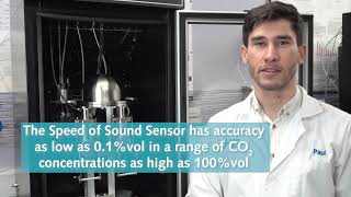

Hybrid Workshop: Measuring Material Vapour Pressure Properties Using Advanced Sorption Technique

PCL Hybrid Workshop: Recent Advances in the Characterisation of Pharmaceutical Powders


Using Advanced Techniques to Test the Performance of Recycled Bathroom Tissue | A video summary