Scientist Stories: Chris Johnson, Single Molecule Spectroscopy
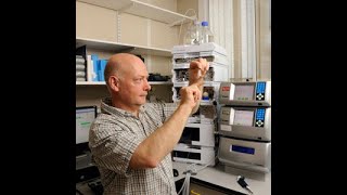
Chris Johnson explains single-molecule spectroscopy, which measures individual molecules to reveal hidden dynamics and rare states. He walks through the LMB's confocal microscope setup and three applications: FRET on a fast-folding protein that shows a two-state barrier, FCS on peptides that exposes nanosecond dynamics, and mass photometry for label-free protein complexes.
Chapters
So today's topic that I'm going to try and cover in some level is on single molecule spectroscopy. And the first— I can't— OK, that's strange. I can't change slide anyway. OK, so the first question that you might ask yourself is why would you want to measure single molecules? You may be working in the lab with a few microliters or a mL of a solution of your molecule of interest at micromole level or thereabouts, and within that sample you have 10^12 to 10^15 molecules. And so when you're making your measurements with the that sample, you may stand there and think, do I really want to make these measurements 10 to the 12 or 10 to the 15 times harder to do? And this slide, I hope, gives you some information about why you would want to measure single molecules. The whole point of observing single molecules is that what we can look at is a distribution of properties within a population. So we can see heterogeneity, as shown here in the, in the red distributions, or a non-Gaussian type distribution shown in the green, or we might be able to pick up rare conformations here, as shown in the light blue. And if we're making a bulk, or what is an ensemble measurement of many, many molecules, then we'll end up observing this average molecular property, and that average molecular property would be observed for all of these scenarios. So we would have no idea about the distribution of properties within the population. If we then add in time as an additional domain, we can start to see stochastic or mechanistic dynamics in individual molecules, And the problem with an ensemble measurement is that all of these dynamics are unsynchronized. So again, here, if we— if this was a property of our molecule of interest that was oscillating between two values, then we would end up in an average measurement measuring this value and have no idea about these fluctuations. Another feature about single molecule measurement is it allows us to pick up rare events or low populations of species which may be biologically important. And from a kinetic standpoint, if you make ensemble kinetic measurements, the actual order of events can be ambiguous, whereas in single molecule events you're able to observe this as a, in this case, an on-pathway event between these two states. So these are pretty important and very powerful aspects of single molecule measurement. And one thing to just clear up is when we talk about single molecule measurements, people often think that we're talking about just measuring one molecule, But in general, all systems that are behaving in a statistical manner should follow something known as the ergodic principle. This meaning that if we average many molecules, just as we do in an ensemble spatial average, or what we can commonly call a bulk measurement, this is equal to averaging the behavior of individual single molecules for a long period of time. So we would look at one molecule for a long, long period of time. That's a temporal average, or many, many individual single molecules, but each for a short period of time in a numerical average. So measurements that we make in solution, which we call single molecule, are not typically performed on one single molecule. Observed over a long period of time. More usually, the single molecule data is the collation of many single molecules which has each been observed individually for a short period of time. And the reasons for this, as you'll see later in the talk, is because of rapid diffusion of molecules and also photophysics of the labels that we might be using. However, the really important point is that the properties of the molecules are observed one molecule at a time. So we can think about many techniques that we could apply that actually probably could be defined as observing single molecules, and a very popular technique at the moment, and obviously very much in favor, is is direct observation using cryo-electron microscopy. The disadvantage of this is what you get is a snapshot, or a view, or a structure of your molecule of interest. You may get a number of different structures in different class averages, but essentially these are— I don't want to use the word frozen, but they are frozen views of the molecules. X-ray crystallography probably doesn't seem like a single molecule method, but effectively, by ordering molecules in a lattice, you're effectively generating a giant version of the molecule that gives you sufficient intensity of scattered X-rays. Again, you get a very largely static view. You can look at B-factors, but basically there's no information about different structures or dynamics within the system. We've also heard in the first 4 talks in this series about imaging, and in particular super-resolution microscopy, which is approaching molecular resolution and being able to observe individual molecules. One of the problems with this is that you have to fix your sample. Again, it has to be not moving while you're acquiring the data. So the first— fourth option, sorry, in terms of observing single molecules might be to apply classical in vitro spectroscopy. And in that process, we're looking at freely diffusing or immobilized molecules, and these can undergo stochastic and mechanistic dynamics in solution. And by using simple solution spectroscopy, we're also able to apply biologically relevant conditions and control conditions in terms of solvent and temperature. The other advantage of in vitro spectroscopy is it tends to be a lot cheaper to initiate in a lab than these other techniques, and there seems to be a very strong inverse correlation between the cost of these techniques and their general availability and the speed of data acquisition that you can perform. So we've talked about dynamics, and one of the things that's quite important to bear in mind when we see these very elegant structures— this is a structure determined by X-ray crystallography in the LMB, and here's a cryo-EM structure, and here's some super-resolution imaging pictures, or picture, and obviously these convey to us a very static and fixed view, but at atomic resolution, of the biological system of interest. But we all know that in the real world we have a lot of dynamics going on, so within the cell we've got molecules diffusing by Brownian motion within the cell, or they may be diffusing under energetic or mechanistic methods, being transported. We also have huge elements of molecular crowding that we shouldn't forget, and then when we come down to individual molecules, they're undergoing dynamics on, on a huge range of time scales, And here also is the participation, or the incorporation of solvent within the observation of this molecule, and solvent is something that I'll discuss in a bit more detail in the talk about calorimetry next Tuesday. But essentially, the point here is that dynamics are going on all the time, and they're an important part of biology. So having methodologies that allow you to observe them is really very an attractive prospect. So what are the strategies for making single molecule spectroscopy measurements in vitro? So these are kind of an approach that we will have to take in order to be able to observe single molecules. So the first thing that we— and a common feature of single molecule measurements is to dilute the sample. So we want to reduce the concentration such that statistically we're only observing one molecule at a time. So typically we're going to be working in picomolar to nanomolar concentrations. And this has some advantage in that a very small amount of protein can go a long, long way in terms of a single molecule-based project. We also, as well as diluting the sample, we limit the observation volume, so we try and reduce the volume that we're collecting data from, and using diffraction-limited confocal configuration, we reduce volumes to the order of femtoliters and also try and reject as much out-of-plane signal, as, as been discussed in the earlier talks. We can also use TIRF illumination microscopy, and that restricts the observation depth to some 50 to 100 nanometers from the glass surface. We then would localize the system of interest at a low density in this layer. So if we look at the confocal condition, we have 10^-15 of a liter, and say we're working at picomole, 10^-12 molecules per liter, so we're down to 10^-25. So we should be working at a true single molecule level. Some other things that we do when we're doing single molecule spectroscopy is we will use strong optical signals, so we tend to use bright extrinsic fluorophores with very high quantum yield, and these are typically excited at visible or longer wavelengths. The reason for using longer wavelengths is it reduces scattering, and light scattering has an inverse relationship to wavelength, and I'll talk about that later in the series in the light scattering talk. And finally, we also use strong illumination sources such as lasers, and lasers can give problems with very high illumination fluxes, and we can get a lot of photobleaching, so we should bear that in mind and also, if we can, consider using multiple wavelengths. So some practicalities that come out of these approaches and single molecule methods in general. We have to consider if we're going to start using extrinsic fluorescent labels that we're putting onto our molecule of interest, that this may perturb the system, and the fluorophores may also go complex photophysics at the very high illumination intensities that we're going to use with laser illumination. So we often need lots and lots of controls to quantify the system properly. So when we come to looking in vitro at purified materials, then single fluorophores or multiple fluorophores at defined labeling sites is definitely the cleanest approach and produces the most unambiguous data. So to obtain those labelings in defined positions, we may have to do some mutagenesis on our system, or we may have to resort to using fusion proteins. And labeling strategies were covered in some depth in the third talk in the series. Within the LMB, the instrumentation that we have is home-built, or I assembled the instrumentation, which is actually just behind me in the room that I'm in. And it, it requires some expertise to build. It's not particularly difficult, but to construct and maintain it and obtain optimal data requires some level of expertise. Single molecule concentrations, as we've discussed, may be very low at picomolar to nanomolar, and this may not allow stable complex formation of our system of interest. There are ways around that by using, adding additional unlabeled material, which increases the overall concentration but not the concentration of the molecules that we can see using fluorescence, for example. And also, at very low concentrations, we have to be aware about nonspecific absorption onto surfaces and this can be a problem if we're interested in the diffusion of the molecules. And finally, if we want to look at events that are on a reasonably long time scale within a single molecule, such as the stochastic fluctuations that I showed on the first slide, then we might require to immobilize our molecule of interest in some way or another. And again, we have to be aware that this may perturb the system, so again, more controls may be required to verify that. So single molecule experiments, when you come to thinking about doing them, should be a very logical approach that's required for your project, and the experiments should be well designed, and they should try and target a specific tractable question, because you may have to undergo some amount of additional work to get to the, to get to the point where you can make the measurements. So I've mentioned already that we can look at freely diffusing or immobilized molecules, and one of the issues here is that with a confocal volume of micrometer or so, then diffusion through that confocal volume by a random stochastic process is going to occur on the order of milliseconds, depending on the size of your molecule, the viscosity of your solvent, and, and various other elements of the optical configuration of your system. So for this reason, we can use very high illumination intensities because photobleaching may not occur over this very short time scale of a few milliseconds but the transit time through the confocal volume is very short. So if we're interested in processes that occur on a slower time scale, then we may need to consider immobilizing the molecules. So observing these requires immobilization. Another approach that you can use, apart from immobilizing your molecules on a surface, is to, is to have an immobilized biological scaffold presented in solution that the, your molecule of interest can interact with, and this is implemented in a technique called optical tweezers. The confocal approach can target either diffusing or localized systems, while TIRF illumination is obviously predominantly a technique that you would apply to systems that have undergone surface capture. So in just talking about diffusion and showing you a movie where we see molecules diffusing around it, I just thought it's interesting to think about the timescales for a stochastic diffusion process. And if we think about a molecule traversing a distance x, this is related to a property of that molecule the translational diffusion coefficient, which for a typical protein, or say a 30-kilodalton protein, is around about 10 micrometers squared per second in, in viscosity of the cytoplasm. So the time for a three-dimensional diffusion of that molecule is x squared, the distance, divided by 6D, which is 6 times the translational diffusion coefficient. So why that's interesting is that if we start to think about diffusional times over a different length scale, so for example an E. coli, which is a micron or so, it will take 10 to 20 milliseconds for that 30-kilodalton protein to diffuse from one end to the other by a random process. You start thinking about bigger cells, it might take 10 seconds, And then if we think about a neuronal cell, which is about a centimeter long, this can take potentially 20 days for random diffusion of that protein from one end of the cell to the other, or over that, over that length scale. And when we consider a sciatic nerve, which is about 150 centimeters long, I'm told, then that equates to 71,000 years. Obviously, this is the reason why cells have evoked specific transport mechanisms where molecules can be directed in, in specific directions and at reasonable speeds, rather than relying on random diffusion processes. So in the buffer, which is obviously a less viscous environment than the cytoplasm, D, the diffusional coefficient is about an order of magnitude faster, and so therefore the transit time for random diffusion in a confocal volume is about 2 milliseconds, as I've already said. And so if we consider a fluorophore that's giving us a count rate of about 10 kHz in terms of photons, that fluorophore will yield about 20 photons during its transit time through the confocal volume. So this just emphasizes that single molecule experiments are actually quite, quite technically challenging to perform. So obviously these talks are specifically aimed at people in the LMB, although we welcome people from outside the LMB in the Cambridge community to join and, and get some information about various biophysical methods. But what I'm going to do for the rest of the talk is just consider some of the instrumentation that we have in the LMB and show you some of the work that we've done with this. So there are various types of single molecule techniques which— and you can kind of characterize them in terms of the, how they're applying a particular physical parameter to your molecules of interest. And there's a whole group of single molecule techniques that are based around force or manipulation, and atomic force microscopy, which uses a probe which you either tap or, or drag across your sample of interest, and monitor the deflection of this probe. You can also use them in pulling mode. We actually have an atomic force microscope which is set up for biological measurements under, under liquid in the LMB, but I'm not going to talk about that. And if you have any interest in that, you should talk to Nick Barry, as it's part of the imaging facility. We're also in the biophysics facility very interested in optical and magnetic tweezers. We don't have that instrumentation, but we're strong— we're trying to develop a case for having that technology within the LMB. And in that approach, you have a polymer such as DNA which is held between magnetic beads and/or under beads that are held in optical traps. With using lasers, and you can apply force or watch molecules move along those polymers. The techniques that we do have here at the moment and that are set up are optically based. So we have a lab-built confocal fluorescence microscope-based instrument, and this allows us to make FRET measurements, and FRET has been discussed during talks 3 and 5 of the series, so I'm not really going to cover any of the details of FRET. I'm going to assume that you know, know what that is and how it occurs and what you should think about in designing FRET systems. And this can be used to measure populations, distances, and so forth. And with this confocal setup, we can also perform a technique called fluctuation correlation spectroscopy, or FCS. And this allows us to measure diffusional times. One can look at interactions between molecules, which lead to a change in diffusional time, and we can also look at fast time-resolved intra-chain dynamics using an adaptation of the FCS technique. The other optically-based system that we have is a commercial instrument made by a company called Refine, And it's based around interferometric scattering, which allows us to measure instrument— allows us to measure molecular mass. So in the remainder of the talk, I'm just going to describe the instrument that we've got here and show you some examples of FRET measurement, FCS measurements, and then finally come on and discuss the iSCAT instrument and show you some data from that. So first of all, talking about the instrument itself, this is the configuration of the instrument. It's homemade or lab-built and is— it's quite flexible for that reason, but it tends to be a bit temperamental and quirky. So over here on the, on the right, we have a series of lasers that are used to illuminate our molecule of interest, or our molecule carrying a fluorophore. And these lasers are combined through a series of optics into a fiber optic. We then process the beam coming from this, we collimate it and control the aperture of it, and then this is directed into the objective of a conventional confocal microscope. This gives us a diffraction, or the way it's configured gives us an observation volume around about a micron in diameter, and we can look at freely diffusing molecules in the picomolar to nanomole concentration range. In terms of the data that we can collect, we can use the prism within the microscope to direct the photons that we collect from our sample either into an FCS-based system where we have a beam splitter, and then we have two avalanche photodiode detection systems. And this allows us to do cross-correlation between these two photodiodes, and this removes potential artifact which is called afterpulsing, from the photodiode signal. And this is particularly important when we want to look at sub-microsecond dynamics. On the other side here, we have a configuration for measuring FRET, and here instead of a beam splitter, we would have a dichroic that would separate the donor and the acceptor photons that we want to count. So here's some views of the instrument. It looks somewhat simple on the schematic, but obviously in reality it's a bit more complex and involves lots of sort of giant LECO pieces. Here are the lasers. Obviously we don't operate it in this mode with unshielded lasers. This is just for the purposes of the photograph. In terms of samples and how we put our systems of interest onto the instrument, this kind of confocal setup is compatible with pretty well any buffer at all. In terms of surface absorption problems, we can either passivate the glass surfaces—that would be either a coverslip a slide with a coverslip on it, or these so-called Tek trays, which are kind of plastic trays with a coverslip, optical coverslip, as a base. We can passivate the surfaces using polylysine, or we can include other molecules that reduce nonspecific surface absorption if that's a problem. So I've said we can either use these kind of dimpled slides, takes about 20 microliters to fill, or we can use these Tek trays. And in the 8-position Tek trays, takes about 200 microliters to— is required of our very dilute solution. The trays are particularly good because it's a relatively large volume. We can just remove the lid of the tray, and then we can add in other components and carry on measuring. So we can do titrations, we can add metabolites, or we can add different biology and perform mixing and then just remeasure. So let's talk about some FRET work that we've done with this system. I'm just going to measure— sort of mention something about an application where we used FRET to address a question in protein folding. And protein folding is historically obviously a very long-standing problem, but in recent years, you know, after— in the beginning of this century, I should say, so from 2000 on to 2015, there was a lot of argument about whether or not very fast folding proteins which are typically usually very small proteins, or effectively large peptides under 100 residues in size. They fold very, very fast, and there's a lot of argument about whether or not these proteins folded via a mechanism where there was a high-energy barrier, or a transition state between the folded and the unfolded states, or whether they folded via a sort of non-cooperative gradual accretion of structure. The one, the argument where they were folding via a transition state, so-called two-state folding, and then the counter-argument that they folded without an energetic barrier became known as one-state folding or downhill folding. There were a lot of publications on this, and unfortunately, although it generated a lot of papers even in very high-profile journals like Science and Nature, the whole issue was controversial and ambiguous because ensemble measurements were— or kinetic measurements were unable to discriminate between these two models. So, the barrier-limited argument was sort of supported by observations that many proteins fold slowly and definitely do fold over large energetic barriers, and it would only be the very fast folding proteins that would have this particularly unusual mechanism. And equilibria and kinetics were consistent with activated or barrier-limited cooperative process. And one could also imagine that biology might actually require a distinct active and inactive conformation to allow it to have processes of evolution. If you think about a downhill, or no barrier, or a gradual accretion of structure, it may be difficult for biology to work with systems that are kind of partially active when you make mutations. In terms of the barrierless, or downhill, or one-state folding, this was a prediction of energy landscape theory, which was very popular, and was predicted to occur under extreme native conditions. And small proteins do indeed fold very, very fast, in microseconds or so, near diffusional controlled speed limits. So theoretically, they were passing over very small or very limited barriers. And it was also attractive as a proposal because the proponents were suggesting that folding mechanisms could be mapped out at equilibrium because the structure between denatured and folded was gradually acquired over a process of destabilization, and so you could map out the pathway for that event. But the debate continued, as I said, because equilibrium and kinetic measurements were ambiguous. So we decided to look at this system using a single molecule approach, using FRET. The protein we looked at was a protein known as Bbl. It's about 50 residues in length. We attach two fluorophores, Alexa 546 as a donor and Alexa 647 as the acceptor. Here you can see the spectral properties of the two fluorophores. So we're exciting here with a 532 laser, and you can see this is the emission of the donor, and here's the spectral overlap with the excitation of the acceptor, and then here's the emission of the, of the fluorescence acceptor. One of the things that we confirmed initially was that when we made labeled and unlabeled material, the stability of the material, as assessed here using denaturation curve with guanidinium hydrochloride, the stability of the labeled and unlabeled material was, was identical. So that here on the right is an example of what, what data would look like. If you remember, you have a donor and an acceptor APD in the configuration of the system, and they're collecting wavelengths appropriate for those two fluorophores. So we measure the photon counts of the donor and the acceptor, and we average those fluorescence counts over some predefined bin interval. In this case, this is 200 microseconds. And then what we have to do is to set a threshold for an event. So what we're imagining is we're looking at the signal, and in these periods where we have very low signal, there are no molecules diffusing through our confocal observation volume. When a molecule does pass through, we get a burst of photons. We define this burst of photons with some threshold, and that burst level will depend on the— the burst level will depend on various things such as your time binning and your background. And the burst is then classed as a molecular event, and the FRET efficiency of that burst is defined as the ratio of the photons, the number of photons in the acceptor channel divided by the total number of photons counted in donor and acceptor. What you then do is observe many, many of these burst events as a trajectory. You just collect data over, say, half an hour, and you measure many, many bursts, and then you go back, analyze the data, and you can construct a FRET histogram or a population distribution of the FRET efficiencies from many, many of these single molecule burst events. This might look something like this histogram at the bottom, and you'll, you'll, you'll see here that we have something known as the zero peak. The zero peak could come from a donor-only labeled molecule that passes through the observation volume, so that obviously gives a big burst in the donor fluorescence emission. Or it could be that we have molecules where the acceptor is not fluorescing, or, or in some way photo-bleached or damaged. And having this zero peak, if, can be eliminated using more complex pulsed excitation methods of FRET, and if you read in the literature, you may see references to various other applications of FRET. This pulsed interleaved excitation and alternate laser excitation, laser emission excitation methods. We don't have that, and so in our data here, which shows the various FRET histograms as measured, you'll see that there's quite a strong zero peak present in the data. However, in terms of the FRET that we're interested in, it's all occurring at much higher FRET efficiencies. And Stephen spoke in the last talk about how you can use denaturants to simply alter the stability between the native state and the denatured state at high denaturant concentrations. Simply by changing concentration, and that's— this has a somewhat linear effect on the free energy of the system. So at low guanidinium hydrochloride concentration, we saw one single FRET distribution of high FRET efficiency, corresponding to the two fluorophores being close together and being able to FRET with high efficiency. And here you can see the location of this FRET peak remains pretty constant at low guanidinium, where we only have the native state populated. As we start to go into this transition region, we would expect in a barrier-limited system to have two distinct or discrete states populated, and that's exactly what you can see as we go further into the transition region. You can see that the native state decreases, and this denatured state corresponding to the molecule being unfolded, the fluorophores are further apart, and therefore the FRET efficiency is significantly reduced. This denatured peak starts to build in, in amplitude, and eventually, as we get to very high denaturant concentrations, we essentially have only one species. So this bimodal distribution of FRET efficiencies strongly supported, in our opinion anyway, this two-state folding mechanism, and went against an idea of having a one-state or gradual accretion of structure, where you would expect to see a single peak that would move in FRET efficiency as you denatured the molecule. Unfortunately, that didn't prove to be the case, and the argument about two-state versus one-state folding still continues, but that's another story. So coming on to fluctuation correlation spectroscopy, which can be used for measuring diffusional times and looking at interactions. This is typically what the signal coming from the APD might look like, and we have to consider how we're going to measure and analyze these fluctuations. So molecules that pass in and out of the observation volume cause fluctuations, cause fluctuations in the signal at the detectors, and these fluctuations are typically analyzed by calculating the autocorrelation function, or the autocorrelation of the signal, for different offsets in time. So, you can see here's the formula we would use. So, you have the fluctuation in intensity at time t, and this is multiplied by the fluctuation in intensity at a longer time, generated by effectively taking the data and offsetting them by a very small time increment, and this is normalized relative to the average intensity. So as we begin to have increasing offset in time, obviously with no offset we get perfect correlation between the two datasets, that being the original dataset and the offset dataset. And then as we progressively offset the data, the second dataset relative to the original one, in time, we get a progressive reduction in correlation between the two data. This then leads to a correlation curve where we go from a high level of correlation down at very long times of offset to no correlation at all. Fortunately, we have small electronic boxes that are able to perform all of this numerical work in real time during the data collection. And as I mentioned earlier, if we use two APDs, we can ask the hardware here to perform cross-correlation between the detectors, and this increases resolution by removing this phenomenon of afterpulsing. In the data. So here's a, a FCS correlation curve, and what we get is both an intensity plot shown up here at the top on the right. This is just the intensity or the photon counting rate from the two APDs. So we can look at intensity, we can look at bleaching, that would be a decline in signal. We can look at quenching, and we can also observe the labeling efficiency of our labeled sample. When it comes to the autocorrelation function, which is done, um, as described previously, we can analyze this and fit this to get a translational diffusion time here, and we can also obtain the average number of particles in the observation volume at any one time. This, this comes because this is a Poissonian statistical process, and what we're doing is effectively dividing— this product of the fluctuations here is the variance, and we're dividing, which is equal to the average for a Poissonian process. We're dividing this by the average square, so we effectively end up with 1 over the average, which reflects the number of particles within our observation volume. You can fit the data either to a 2-dimensional diffusional model or a 3-dimensional diffusion model, and usually a 2-dimensional model does pretty well, because the aspect ratio is pretty large in terms of the z dimension being much larger than the xy dimension. Okay, here's the fitted data. You can see there are about 90 molecules on average in the observation volume, and then here is the translational diffusion time in milliseconds, so about 800 microseconds. One thing just to point out is that although we've talked about FCS being a single molecule technique, we can work with some number of molecules on average within the observation volume, but obviously the fluctuations which originate are the property of single molecules, and so they only depend— the fluctuations only depend on the transition, the translation of individual molecules, and not on the other molecules that might be present. So we typically work around a microensemble of 50 molecules or so. What we can do with the translational diffusion time is to calculate the hydrodynamic radius, And you can do that if you can calibrate the instrument to measure the observation volume, or more simply, if you measure the translational diffusion time of a known standard. And here you can see where we've measured on our system some hydrodynamic radii, which is derived from the translational diffusion coefficient using the Stokes-Einstein equation. You can see that we get very good agreement between the measured values on the FCS and those measured using other techniques. So then we can also think about what happens during the transit, or during the diffusion of our molecule through our observation volume. What happens if there are additional fluctuations in our fluorophore intensity. Well, obviously, if there are additional fluctuations, these will be analyzed by the autocorrelation analysis. And so what we can see is we have a diffusional time in the order of milliseconds, and we have faster kinetics or faster processes going on which originate from additional fluctuations that are occurring when the molecule is passing through our observation volume. Excuse me. And there's a technique which is called PET-FCS, standing for photo-induced electron transfer FCS, and this specifically uses a group of dyes based around oxazine chemistry, and these oxazine fluorophores are very effectively quenched when they come into van der Waals contact with either tryptophan residues or guanine residues. So this is a very nice way of generating additional fluctuations, because these are going to be possibly intrinsic to your biology of interest. So we can start to look at intra-chain and inter-chain contact formation. So the application that we had for PET-FCS, flux, for this, and for FCS, was to have a look at some peptide dynamics, and this came out of an increasing reduction in size, or an approach that's been pioneered here at the LMB, where the original therapeutic antibody approach by Cambridge Antibody Technology was later reduced down to a single domain antibody, as in the company Timantis, and then eventually the actual CDR region was displayed as a cyclised peptide using phage display during a selection process, generating these bicycle peptides, and that's led to another company, Bicycle Therapeutics. The advantages of bicycle peptides were proposed to be that they were more constrained and less dynamic, and as a result, there's possibly a smaller entropic penalty when they bind onto targets relative to an unconstrained or a linear peptide. They should be more protease resistant in that they're structured and potentially have better tissue penetration. So there was a bicycle peptide. Here's the sequence, and here's the structure, the chemical structure of this peptide. Here you can see the bicyclic chemistry that leads to the name of bicycle peptides. It's a thio-based cross-link. So this particular inhibitor of calicrine was evolved using phage display and showed an IC50 of a couple of nanomoles, and this was very favorable when compared to The same sequence for a linear peptide, which was on the order of IC50 of 10 micromole, and it also inhibits coagulation ex vivo. So it all looked very promising. The argument again was the pre-constrained peptides— we've lost a lot of entropy relative to a linear molecule here— they would bind tighter, and they're less dynamic, and that was the reason for their tighter binding. But when looking at them in NMR, it was evident that in terms of NOEs, they could not see any NOEs at all. This was not consistent with the proposed rigid structure, so we used FCS to have a look at this system. And here is the design strategy. We have a linear labeled peptide with a phenyl aniline at this position, and then we introduce the dye here. We can substitute the linear peptide with tryptophan, have the dye in the same position. We can then have a monocyclic version of this peptide, which is cyclized here with a single link, and then a bicyclic version of the peptide. Again, these both have the tryptophan quencher in the, in the sequence., and then here is the unlabeled bicyclic peptide. So what did we see by FCS? Well, we saw, if we looked at the dye alone, we saw simple diffusion of our oxazine fluorophore. And then again, when we looked at the linear dye— sorry, the linear peptide here without any quencher at this position, without the tryptophan, so we have phenylalanine. Then we again see just simple diffusion. Obviously, the diffusion is over a longer time scale because we're looking at not just the fluorophore but a 17 amino acid length peptide, so diffuses slower. Then when we came to look at the linear peptide with the tryptophan and with the fluorophore, we can see some massive additional dynamics, which is exactly what we expect on a time scale of about 100 nanoseconds. And this is very consistent with literature values for the separation in sequence. Obviously, we have a proline in the middle here, which complicates things a bit, but nevertheless, this time scale for a linear peptide intra-chain contact formation was consistent with the literature. When we look at the bicyclic peptide, which was the one we were interested in, we see much more moderated amplitudes of PET fluctuations during the diffusion, and these are on a slower time scale. And so, this was fast enough to explain why we were unable to see any NOEs by NMR, We also had a look at the cyclic peptide, and this behaved somewhat more unusually, in that the diffusional time of the cyclic peptide was longer than the bicyclic. So we're imagining that within this monocyclic peptide, there was some sort of levels of collapse that allowed it to diffuse over a different, more timescale. So that was rather rushed, and I'm aware that I'm running out of time. Here are some more examples of how we've applied either FRET or FCS within studies in the LMB, including some interesting work on spider silk protein, and various other studies that look at dynamics of small molecules, but also some work on some much larger molecules with people in neurobiology. So in the final 5 minutes, I'm just going to talk about the technique of iSCAT, which is an interferometric scattering method. So in this technique, what we do is we look at macromolecules in solution that are diffusing, but they approach and are absorbed onto a glass surface, and these molecules act to scatter the— some of the incident light, shown here as this in this cone EI, and the scattering light ES can be optimized so that it interferes in this case destructively, with the light being reflected from the glass-liquid interface, which is this light ER. So we adjust the optics so that the scattered light interferes destructively with the reflected light, and there's a lot of very complicated and proprietary optics going on within the instrument and careful numerical aperture filtering, which is described in some detail in this paper. And this allows the contrast that's generated by this molecule, by the interference between the scattered light and the reflected light, to be measured. And this contrast that you can see here that arises as the molecule lands on the surface. This contrast will scale linearly with mass, so we can measure macromolecular mass. And we can also, by looking at this property over very many events or very many landing events, we can look at the heterogeneity of this mass within a population. So the system uses a camera and has a fairly large field of view. Field of view, which is obtained via a scanning mechanism, and this allows very many events to be observed pretty rapidly within a fairly short acquisition time. And light scattering is actually a universal property of all proteins and all other, or most biological macromolecules, and it's a function of their polarizability, and I'll talk more about that in the light scattering lecture later in the series. The important point though, therefore, is that iSCAT is a very universal technique, and it also requires no label. This is purely— the scattering is purely a property of the molecule itself. So here's the instrument that we have in the LMB, made by this company called Refine, and they like to call the technique mass photometry rather than scattering interferometry. The nitty-gritty is that you need 10 microliters or so of sample, and you can work in this concentration range. I've just said it's label-free, re-emphasize that. And what you do is you take a very clean glass coverslip. You can apply a silicon gasket, which is optional. I've used just a method of applying drops directly onto the coverslip. That works well. And then there's an oil objective lens that comes up underneath, collects the data when the laser is turned on, and we end up with this series of landing events within the field of view. And I think here you— so this is an actual movie coming from a data acquisition. So we can observe many landing events in the movie. We're recording at around 100 frames per second for 1 minute. The frames are then averaged and we generate a running ratio, which is calculated by comparing frames from before some time point to frames after the time point. So-called ratio metric view. So therefore what we see, and what you see in the movie below, is that molecules— the molecules appear and then they land and then they then disappear. The reason for this is once they are stuck onto the surface, as they do in most cases, then the molecules are scattering light in the frames before and after the time point. So therefore, when you take a ratio metric view, they have disappeared. But as they approach the surface and land on the surface, we see these characteristic landing events. The contrast— sorry, the contrast generated is negative since we're looking at a destructive interference effect. With the bulk reflective light, and multiple events can occur at the same position on the coverslip in the movie. And because we're looking at sub-diffraction-limited process, the molecules are much smaller than these points that we're seeing in the movies. The software will then analyze discrete non-overlapping events, and then it evaluates the maximum contrast for these individual events. You then convert the contrast that you've seen in this ratio metric view to mass using a calibration curve. And then how do you use this technique? Well, we can look at mass determined in solution and look for heterogeneity of population. We can confirm, which is very useful, the assembly and stabilization of complexes. In particular, for cryo-EM work, we can very rapidly confirm that we have the expected mass of the complex before we embark on a cryo-EM session, and we can also try and look for conditions where that complex might be most stable. It's very quick, it takes minutes only, and we're working in the nanomole temperature— nanomole concentration range.. And again, we need no labels. Here's some examples then, just finally, of some data that we acquired. In this case, confirming here that we have a heterodimer. The two subunits in this heterodimer would have a mass here, so we can see that we have complete population of this heterodimer. And here's another example where we're looking at a homodimer. Here we're looking at stability of a homodimer. In this case, at the concentrations measured, we start to see the, the dimer dissociate into subunits. So here are the— here is the subunit mass. At higher concentrations of 100 nanomole, we have a lot more of the dimer than the monomer. And then as we reduce the concentration to 40 nanomole, we can start to see roughly equal amounts of monomer and dimer. And then very finally, here's an example of some work that went on for cryo-EM studies. In this case, these blobs represent a 15-subunit structural complex of a massive biological machine, and for structural and mechanistic work, it's very important to confirm that you have all of the subunits present and present in solution. So here you can see the individual expected masses and the theoretical masses are, are pretty close, and we're able to determine the addition of small additional subunits onto this large complex. So I'm sorry if I went over time. I'm trying to fit in a lot more than I did last year because we didn't have the iSCAT machine last year. But thanks for listening, and if you have any questions, I'll try and answer them if you put them in the Q&A. And here I will leave this information up just for you to digest, which is a summary of the talk, a couple of references for recent reviews, and where you might also find further information. And for people in the L&B, these are kind of developments that we might want to think about in terms of adapting our system that we have. So we have one question: is it possible to share the slides for the talk? It seems the link to the slides from last year redirects you to an MP3 part. Okay. Yes, okay, the answer to that is please go to the LMB external website and go to the LMB YouTube channel, and if you look on that YouTube channel, you should be able to find the biophysics lectures being put onto that YouTube channel where you can watch them. In terms of if you wanted the slides, you should be able, or possibly able, to access the slides from the talk from last year, but I'd have to look into whether or not if you're coming from outside of the LMB, whether you can access that. The best thing then is to please email me directly, and I will address your issue in terms of, of that. So any other questions at all? All right, well, thank you again, and we'll perhaps see you next week for changing tack completely, looking at calorimetric approaches.
More from Joshua







Scientist Stories: Hans Waterham, The value of phenotypic assays in peroxisomal disorders




Scientist Stories: Joel Zlotogora, Genetic carrier screening programs for reproductive purposes