Scientist Stories: Christian Eggeling, Super Resolution Microscopy in Biomedical Research
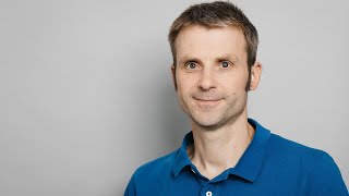
Christian Eggeling explains STED microscopy, which uses a donut-shaped laser beam to shrink the diffraction limit down to 20 nanometers. He shows how STED-FCS maps lipid movement in cell membranes and HIV particles, and describes emerging techniques like MINFLUX that track fast molecular motion without heavy photon demands.
Chapters
—quite a few years through the— I'll just start that again. So welcome, everyone. Today we're very lucky to have Christian Egeling talking to us from Jena. And I've known Christian for quite a number of years. And we've had some great interactions at the Plymouth Microscopy Course, which has been a great place to go and sit by the sea and do all things microscopy. So Christian hangs out in many places between Oxford and Jena. And I'm never entirely sure where he is at any one point, but hopefully other people are. And I've visited his labs quite a few times, a few times, and he's always really enthusiastic showing off his latest technology, especially the latest lasers and other equipment that he's been developing. So, and I'm sure Chris can be able to give a better introduction of himself than I will, so I'll hand straight over and we'll move on.
Yeah, thank you, Alex. Yeah, I hope that we have Plymouth going on at some point again, so I would be looking forward to come to this lovely place at the sea again. So I always enjoy going there, and I also, I mean, I've been in Oxford before. I'm slowly closing my lab there. Before that, before I came to Oxford, I was in the lab of Stefan Hell, of course, developing all these, these step microscopy techniques and stuff like this. But the most important part of these techniques is to make them usable. Yeah. So we have to try them out. Do they really work? And what do we have to do to really make them work in real life science research? And that's what I did in Oxford because I joined the medical department and now I'm in Jena, mainly also for private reasons. But also Jena is a famous optics city. Zeiss is here, but that's where Abel was, was working and so on. And that's why I enjoy it really much. There's a lot of biological applications where we can test all of this stuff.. And I'd like to tell you a little bit about this, the challenges, the potentials that we face here, but especially I want to give you a little bit insight into also mainly STED microscopy and later on at the end complementary techniques closing up my talk with MINFLUX microscopy. So super resolution microscopy, yeah, what is it about? Well, this is the famous monument in, in Jena where I'm now teaching and researching. And it's Ernst Abbe, and this is the diffraction law, diffraction barrier. And this is written in stone and it's a physical law. And that's why there have to be tricks to surpass it. And why do we want to do this at all? Why do we want to go to scales that never explored before? Well, of course we can understand a lot out of ourselves when we just look at our body with eyes. Look inside. But the most we learn, and we have to understand to really treat human diseases, we have to understand how molecules interact. So we have to zoom into the cells, we have to understand how cells are built up, and most importantly, how molecules interact. So we have to go from the centimeter range down to the micrometer and nanometer molecular level. And that we can do with microscopy. And when we observe microscopes, we have to observe the a living cell. So we have to be non-invasive. Because while we observe it, we don't want to change anything. And a good way of doing this is with minimal invasion. I'm not saying it's non— completely non-invasive, but it's minimal invasive. It's light. We are surrounded by light. And also going into the far field. Far field means we work with focused light. When we work with focused light and lenses, everybody knows we create a focus. And the focus is usually micrometers, millimeters, centimeters away from a lens. That's why we don't touch the sample, and we can go inside the material. We can go inside an organism, we can go outside the cell, and so that's called the far field. Now the problem is when we work with focusing light, that the size of the spot that we create, or how we call it, the point spread function, is limited by the diffraction of light. Why do we have diffraction? Because we have an opening here, and every time we have an opening, and a lens has an opening, When we have an opening, we have diffraction. Due to this diffraction, we cannot focus light infinitesimal small spots. And that exactly is given by the famous equation of Ernst Abbe. It's given by the wavelengths of light and the opening angle or the focusing strength of our objective lens. And usually for visible light in the lateral direction, this is around 200 nanometers, and the axial direction is around 600 nanometers. And that's exactly here. This is the equation. This is written in stone here in Jena. And written in stone, I mean it. It's a physical law. It's given by diffraction. You can't change the physics. And with that, if we have such a big size, we want to distinguish nearby objects that are closer together than 200 nanometers, they will appear in our focus at the same time. And that's why they will appear undistinguishable. And that's why we cannot distinguish alike objects closer together than 200 nanometers. Now, the good thing is we have fluorescence, and we work a lot with fluorescence. Fluorescence means we use labels that we can excite with laser light, then they excite to higher excited states. And when they fall back down to the ground state, they emit light, and that's fluorescence. And this can be of different colors, can be specific for a certain label, a fluorescent label that labels a certain protein. And that's why we can look at the distribution of the labels in cells. And then we can look at the distribution of the proteins or whatever we tagged in the cells, like the cytoskeleton here or the nucleus here. Now, why does this help us? Well, as I said, this one is written in stone. It's a physical law. How do we get still to distinguish alike objects closer together than 200 nanometers? Well, we can work with fluorescence. We can turn fluorescence on and off. For example, we can turn off all fluorescent objects, but at a single point. This single point is very, very small, and then we scan the single point over the sample, and then we can distinguish alike objects closer together than these 200 nanometers, which I kind of envisage here and as a, as a red circle. Or we can turn off all fluorescent objects but a single object, and then one single object after the other. And with this, of course, we turn on fluorescence one after the other. Nearby objects. We can distinguish them because they show up sequentially. That's why our effective observation area or resolution is smaller than these 200 nanometers. This one is the principle of Storm-Palm, and this one is the principle of STEDS. So let's focus on that because I promised you to go into STEDS, and that's how I grew into super resolution. What do we have to do? Find a way to of depleting fluorescence everywhere but at the center. Very tiny little objects. So inhibit fluorescence, turn it off everywhere but at a tiny little spot. How can we do this? Let's take a confocal scanning microscope. Excitation laser focused onto a 200-nanometer large spot. Within these 200 nanometers, all the molecules are excited. They're falling back to the ground state emitting fluorescence. This is detected. On a single point detector. We create an image by scanning this spot over our sample and registering the fluorescence we get from each spot. Now we have to get this spot smaller. First of all, we have to switch fluorescence on and off. We can do this with an additional laser. This additional laser is the so-called STED laser. This STED laser is in the— this is the wavelength in green, it's the excitation spectrum of the dye, whatever we look at. And red is the emission spectrum of the dye, what we look at. Usually we detect in this grayish area, and then we come in with a step later with wavelengths that is in the far red of our emission spectrum. But still, if this light hits onto our excited states, the excited molecules, it forces them down to the ground state, thereby stimulating emission which we don't detect. So the spontaneous emission which we detect in this wavelength range is gone because the de-excitation is done by stimulation, not via this path. So if we look at the fluorescence with increasing STED intensity, yeah, we can nicely switch it off. Yeah, by increasing the intensity more and more, the efficiency is higher to deplete this fluorescence. Now we want to do this depletion only in the peripheral part, and that's why we shape our STED laser in such a way, we insert these face plates that they— that the light interferes in such a way that it creates this funny donut shape. So there's nothing in the center and everything in the outside. Now the problem is also, of course, also this donut, how we call it, is ruled by diffraction. So these maxima between here and here are also further than 200 nanometers apart. So how do we quench, how do we inhibit fluorescence also close to the center? Well, we do this because we drive this into saturation, the switch-off. Imagine our maximum would be here. So this is just an intensity line profile through here. This is our excitation spot, this is the inhibition. And now let's say we are here at maximum, here at this intensity. So we would inhibit all the fluorescence here, which is just the side parts here. But here, this intensity is somewhere here, wouldn't inhibit any fluorescence. Now we crank up the power of the STED laser. We crank it up, we go somewhere really way here. So this maximum is somewhere here. Then suddenly this intensity is here, and we inhibit fluorescence even here. So if we crank up the intensity high enough, we inhibit more and more fluorescence along this line apart from the very zero in the center. So the area in which fluorescence is still allowed The more we crank up that state laser power, the more the area in which fluorescence is still allowed gets smaller and smaller. So our effective spots get smaller and smaller, the diameter, with increasing state laser intensity. In principle, in theory, we could drive it on and on if we only increase the intensity of the state laser more and more. It's kind of a square root law that we could impinge onto Abbe's equation. So the spatial resolution is maximized by putting more and more light into the system. So we maximize the light. And with this, of course, yeah, this was our case before. And now we have a tiny little spot and that we can scan over there. Yeah, we can scan it over there and we can now, because the effective spot is so small that nearby objects are now switched one after the other and we can distinguish that. So we can image with sub-diffraction. And this is shown here, for example, and we can tune— and that's the nice thing about STEDT— we can tune the size of our laser or the resolution with the intensity of our STEDT laser. Yeah, this, for example, these are red fluorescent beads, 20 nanometers in size. They are aligned on the COVID glass surface and we just scan over there. And this is the confocal spot. And if we look at the spots, they look blurry. If we make a line profile, they are roughly 200 nanometers in size. Now It's coming with a doughnut and we increase the intensity of our STED laser. And if we increase it, yeah, the effective spot gets smaller and smaller, as I explained to you. If we go to this power, it's only a little bit. We get to smaller spots, 130 nanometers in size. We increase the power even more, 80 nanometer spots, and now suddenly we can distinguish nearby objects. And now we crank it up further, we can distinguish more and more objects. And if we crank it up really high, we get to a spot size of 22 nanometers, which is roughly the crimson bead size, and we can really see the individual spots in result. Of course, this also works in biology with cells. These are, for example, T cells. This is the cytoskeleton of a T cell. This is a 3D recording. This is the confocal recording, and this is the STED recording. And we can do it also in 3D. We can do the confinement also from above, below. I come to this later on in my lecture. And in principle, STED is doable. It's live cell, you can go inside, it's multicolor, you can combine it with two-photon excitation, you can do 3D as I show here. And since stimulated emission works with basically every dye, you can in principle do it with every conventional dye. The issue, of course— sorry, the issue, of course, is you put a lot of light into your system. And that's the biggest criticism about STED, that you, because you put too much light into the system, that you can danger the cell. And so I come to this photobleaching issue later on because it's a very important part. You have to remind, we increase the spatial resolution. The moment you increase the sensitivity, you of course not only increase the desired intensity, which is spatial resolution, but you also increase sensitivity towards bias, towards artifacts. And that's why often at the beginning, especially with STED, and that's the good thing about STED because you get a direct image. That's what I like about STED. If your sample is bad, your labeling is bad or something like this, you get a crappy image immediately. That's why confocal microscopy, maybe the spatial resolution was forgiving to still see a badly labeled sample still good enough, but instead you will immediately see it. And that's why at the beginning, a lot of people said, ah, STED is not a good super resolution technique because it was so cruel against bad samples or against bias and so on. And that's why you have to wage this increased sensitivity also towards artifacts against the increased sensitivity you have with spatial resolution. And that's also one advantage about STED is that you can tune the size of your observations. For example, if you say, oh, too much resolution enhancement, let's say going down to 30 or 40 nanometers, it's good enough, I only need 100 nanometers, then you don't go so in there with so much light. That's the flexibility you have with STED. But you have other tools you can play around with with STED. That's, for example, and that's what we did for years now, and I started with this when I was with Stefan Hell's group. You can look at the mesoscale organization of molecules in the plasma membrane. Now the plasma membrane is the surrounding envelope of our cell. Yeah. And if we look into the surrounding envelope, it's a lipid bilayer. So it's lipids, has a polar head and a hydrophobic tail, and the tails are inside and the polar heads are to the outside. So they're sitting like this. It's a 5-nanometer thick layer And proteins are involved in there. And of course, all the signaling has to go via this envelope, because everything that goes in the cell or out of the cell, any communication has to pass there. And that's why there's the interaction of molecules, the organization of molecules in the plasma membrane is so important. And not only the proteins, but also the lipids. How can we investigate? Well, lipid membrane heterogeneity, We have thousands of different lipids in our body. If it would only be a protecting lipid bilayer, one lipid type would be enough, but we have thousands of different because they take actions. And we have especially heterogeneity in our lipid context spatially. For example, we have certain areas where cholesterol and sphingolipids, certain lipids are enriched. We have heterogeneity in molecular packing, meaning how the lipids are packed closely to each other, how they are ordered. Are they more loosely or are they very tightly packed, how many lipids are within one area. And that of course can compartmentalize cellular processes. For example, there are these so-called nanodomains, often they are denoted rafts, and it's environments, areas in the cell somehow enriched of certain lipids or more packed that certain proteins love to go in there and others rather stay outside. That means there's a local enrichment of certain proteins that can then interact and do something. And that's a neat idea. And can we image this? Can we image this lipid heterogeneity? The problem is, it's very heterogeneous and it's highly dynamic. Lipids move around, it's a fluid system, the membrane, and it's small, smaller than 200 nanometers in size. Yeah, and that's why We often miss spatial and temporal resolution. And that's why there's hardly any direct observation methods. And that's why it's highly debated. And that's why, because it's so small, the heterogeneity. That's why I thought, hey, this is a good investigation field to show, can we do something with our technology? So we started off years ago. This was still during Stefan Hell's time. We took a phosphoglycerolipid, a phospholipid, and the sphingolipids, sphingomyelin. And since we are doing fluorescence, we have to label that. From previous data, we knew from biochemistry data that they show a difference. Sphingomyelin should be more heterogeneous, especially it should be going into these nanobrains or rafts. Yeah. Now, since we are doing fluorescence, we have to label them, and we do label them with Atto647 NX dye. It's a very hydrophobic dye. For example, you can put it on the acyl chain, and then you have a fluorescent lipid analog. And then, of course, this label, you change the lipid, and that's why you have to do thousands of controls. And we did thousands of controls. Does the label really sit inside there? Is the functionality of this lipid still the same with and without lipid, and so on. And that's, we did thousands of controls, and you always have to do this. If you introduce a label, you have to do controls. So how we did it, we put the lipid on a BSA complex, and this deliberately and efficiently delivered the labeled lipid to the outer leaflet of our plasma membrane. And then we went to physiological conditions. And we looked with our confocal and with our STED microscope, we looked on there. These are, for example, Jurkat T cells, PE and SM, and this is PTK2 cells, mammalian cells, P-ENSM. And if you look on them, these bright spots, these are internalized vesicles. But if we look on the membrane, like here, here, and here, and we compare between P-ENSM, we didn't see any difference. And there's two things why we don't see any heterogeneities or nanodomains or something like this. Well, first of all, these things are fastly diffusing. Yeah. So everything is highly dynamic. And we raster scan the surface, maybe our spatial and temporal resolution is not good enough. But more importantly, to see heterogeneities, we have to have a contrast. For example, if we have an aggregation here, then we have to have most molecules sitting in the aggregation or in the domains because we need to see them above the background. Now, if we, for example, have molecules sitting in aggregates but as well sitting outside,. And you will see that we have this for these lipids, and we don't have contrast. And imaging, just basic brightness imaging, is not the right thing because we cannot distinguish between domains and the surrounding. That's why we have to discover something else. And what does tell us, for example, molecules sit in more ordered environments. More ordered environments are usually more viscous, less mobility. So when they diffuse through there, through these areas, we should see differences in the diffusion speed, in the mobility. And that's why we said, let's discover interaction and diffusion dynamics. And you can do this instead of scanning your spot, you can just place your spot on one part of the cell and just wait for the molecules to diffuse there. And now you can go with your concentration of your fluorescent lipid analog so much down that the signal over time that you detect looks like this. Most of the time, nothing is in there because our concentration is so low, no no fluorescent molecule in our spot. So that's why we have this background noise. But from time to time, these molecules diffuse through there and we see this rise in signal, it's the burst moving in, moving out. So what do we have to determine? We have to determine the average transit time of our labelled molecules through the observation area. We know the size of the observation area, that's why we can determine the molecular mobility. Now you can do this very efficiently with the tool called fluorescence correlation spectroscopy. Because what FCS, and that's the abbreviation of this, does is looks at these temporal fluctuations and it calculates the temporal correlation function. And the temporal correlation function gives you a decaying curve where the decay time, yeah, is roughly the characteristic time for the processes causing the fluctuations. In our case, it's diffusion, and the decay time is roughly the average transit time. And with the knowledge of our observation spot area, we can calculate molecular diffusion coefficient, and with this molecular— So how can you do this? What are the expectations? Well, SM, we expect to sit in these domains, and these domains are packed with molecules, just like a raft. Picture this as a raft in a river. Now the lipids, the surrounding lipids, move fast. The river flows fast. But these flow more slowly, so we should expect slow components for SM and for PE, only fast for the phospholipid and the sphingolipid. Now, if we look at the FCS curves, there's hardly any difference. PE a little bit faster than SM, but not very— it is not so strong as we would expect between a raft and, and the river flowing around it. So if rafts are stable floating entities, we should see a huge difference. So there are no stable floating entities. So there must be something else. Well, we see a small difference. What is the reason for this? We have to investigate that closer. And how can we do this? How can we image this closer? Well, we need high spatial resolution, super-resolution STED microscopy. And STED has the advantage it creates an effective fluorescence spot of small size. So suddenly the lipids, instead of moving through a 200-nanometer large spot causing these fluctuations, they cause fluctuations while moving through, I don't know, 30, 50, or 100 nanometer large spot created by STED. In addition, because we want to have spatial heterogeneity, this isn't good enough if we just place our spot at one point. We have to place the spot at several points at the same time. So we have to measure FCS curves and mobility at different points at the same time. For that, we take an approach developed years ago by Enrico Gratton and Michel Dickmann and co-workers, where you just take your spot and you scan it along a line, micrometer long, very quickly. You scan it along this line and you can do this with kilohertz frequency and you can scan it 1,000, 10,000 times during several seconds. And what do you get for each pixel along this line? Because you scan it, the same line, thousands of times along each pixel. What do you get? A temporally fluctuating signal. And this temporal fluctuating signal you can correlate, and then you get a decaying curve for each point, for each pixel along this line. And we can see this decaying curve, we can color it from red to blue, and we can look from it from above. So we have this decaying curve from red to blue, red to blue. Most importantly, we look at the decay time. So we look in the yellowish area,. And if we have, for example, a peak towards longer times, lag times, then these are areas where the diffusion slowed down. So that's why I named it mobility. Now let's look at our phospholipid and our sphingolipid. Yeah, phospholipid, confocal size 250 nanometers in diameter. Ah, there is some heterogeneity now, but not really. Sphingomyelin, already some more heterogeneities, but not very distinct. Higher resolution, 80-nanometer spot, STED, of course, the decays are faster now because it takes the molecule less time to diffuse through an 80-nanometer large spot. But for the phospholipid, pretty homogeneous, so we mainly free diffusion, homogeneous all over the place. It's expected as we— transit time reduction as we expected. Now for the squalene lipid, we have this case. Complete heterogeneous. On one hand, we have areas where the decay is as fast as here. Clearly, we have free diffusion at these spots. But then we have spots where the transit time is very slowed down. So the molecules are slowed down at these spots. And these are, if you look closer at this data, these are trapping sites. So the molecules stay there for a while and then move on. And interestingly, if we deplete the cells of cholesterol or even of the acting cytoskeleton, these trapping sites are gone. So, also, if we record one measurement after the other, so every 10 seconds, for example, we record a measurement. What we see here, the PE, it has some trapping, very slightly, but the SM, it has a lot of trapping, but the trapping sites change. They disappear or appear or they move out of the line and new ones come in. So it's highly dynamic. So the idea is, there's, for example, a protein. It's, for example, linked to the cytoskeleton, and it's not alone. It can bind lipids towards it, maybe with the help of cholesterol. And this is like a glue for other molecules to come in, proteins to come in. And that's why there is a constant exchange of lipids into this area. Some just diffuse through there, but some like the sphingolipid stay there for a while. We can analyze it, it's roughly 10 milliseconds they stay inside, and it's cholesterol and actin-assisted, because if we deplete the actin cytoskeleton or cholesterol, there's no trapping anymore. Is there any functional link to this? That's what we looked. Since I stayed in a medical department in Oxford, we did, especially immunology, and if you do immunology, you do T cells. And T cells, they are special cells of our immune system. They patrol our body and they always look out for something bad, and the bad stuff is presented from other immune cells to the outside world or some other target cells like tumor cells or antigen-presenting cells. So antigen-presenting cells take up a bacteria or virus and present something of this virus to the outside world. That is then recognized by the T cell, especially by their receptors, the T cell receptor,. And when this connection is properly— it's really a bad antigen that is detected here— then huge changes are happening at the T cell surface and an immune cell response is starting. And that of course is influenced by the lipid membrane environment because there are a lot of lipids on the surface. And how can we image heterogeneity in lipid environment? Well, we can image the mobility of the fluorescent lipid analogs. And if we do this also on the T cell, we see these trapping sites. Is there a functional link? Now I have to go a little bit into T cell activation. So I told you already, it involves the T cell receptor. And usually it involves that this T cell receptor aggregates. It forms almost micrometer-large aggregates. And out of these aggregates, other proteins like the phosphatase CD45 are segregated out of it. This is shown here by our collaboration partner Simon Davies in Oxford, who took this, this thing. The red part is where the TCR receptors are aggregated, and CD45 in green is outside this area, is segregated away. And that is important so that the signaling can go on. Now, we did this. We took activated T cells, we activated them on bilayers or on an on a cover glass surface with antibodies binding to the T cell receptor, and then we measured lipid diffusion on the TCR aggregation sites, on these aggregates, and outside on the CD45 sites. If we do this and we look, for example, on the diffusion of the sphingomyelin, we look on the aggregation sites, we see trapping, while if we look outside on— at CD45, we see free diffusion. So clearly the TCR aggregates are specific lipid interaction sites. Yeah. So maybe this trapping that we see here, yeah, supports the interaction of less abundant molecules, and thereby gets them together, supports them to get together and stay together, and thereby trigger cellular signaling. This is really the lipid domain idea that we have. And maybe the question here is, do the lipids take an active or passive role? Do they just support it? Do they happen to just go along with this aggregation? Or do they actively drive proteins to cluster? Probably we have examples of this or that, but that's what we try to explore. Another thing where we can do diffusion— we heard so much about viruses over the past 2 years. We did, for example, measurements on HIV viruses. Now HIV virus is the virus that does the AIDS disease, yeah. When they bud out of an infected cell, in order to get infectious, they have to mature. Certain things have to happen on the virus so that it can infect again the next cell. What is the mechanism behind this maturation? That's what we want to investigate. Maturation especially happens— this is the immature HIV virus,, and it has to maturate. And especially what happens is it involves rearrangement of certain proteins of the inner gut matrix. This matrix, it's a protease, it's an enzyme that is active inside this HIV that happens to cleave it off here of the protein, and suddenly it's released from the surface. And these surface proteins, these ones, they have to aggregate, they have to come together, they have to form aggregates, otherwise it doesn't bind efficiently to the next cell surface where the virus wants to infect the cell. How does this rearrangement of Env occur? How? And the easiest is, of course, how do they meet? How can they aggregate? Well, in this case they cannot move, so they cannot find each other. Now this is cleaved off, they can move and find each other. So Jacob back then, my postdoc in Oxford, he came to me and he said, I wanna investigate the mobility of individual proteins on individual viruses. So measure Nth-molecular mobility of surface proteins on single HIV virus. The problem is, of course, the viruses are smaller than 200 nanometers and there are only 5 to 10 copies Okay, sorry, I just looked into the chat. Okay, the problem is also that Env has only 5 to 10 viruses or Env proteins per virus. That's pretty challenging. Clearly, we have to use super resolution, and that's what we did. We used STED and we labelled the inside of the viruses with a green dye, GFP, and we imaged that with confocal. Because we just wanted to find the viruses. We put the individual viruses on the COVID glass surface of the microscope, and then we labeled the surface, the end, with an orange dye, AverioStar 635P, and we used it with STAT. And now we want to look at mobility. Now we have to do FCS. So this is how it looks like. Green, the individual viruses, and in red, with higher resolution, we can look at the distribution of the antibodies. And now we do scanning stat-FCS. We scan along a line over a virus and we scan multiple times. And what kind of signal do we get over time? In the green channel, we of course, we see GFP in the confocal. We know there's a virus here. And on top of the virus, of course, we see the fluctuating signal of the Env proteins moving in and out of our sub-200 nanometer size focus. And then we can calculate correlation function and we can look at the correlation at the virus and outside the virus. Outside the virus, of course, we don't have signal. So we look at the FCS curves on the viruses. That tells us how fast does the end molecule move. We did controls. These are the decaying curves. This is the mature virus, red. In blue is the immature virus. And you already see it's a shortening of the transit time, gets more mobile. But of course, we want to know, is this only photobleaching that we see the decay? Because after a while, the signal is gone. It appears, and if it's photobleaching, it's just photobleaching. That's why we took mature viruses and we fixed them, no mobility. So this is pure photobleaching. You can clearly see we really see mobility. And now we can look at the diffusion coefficient. And this is here, this is the mature virus, this is the diffusion coefficient. Of the mature virus, and this is of the immature virus, and you see an increased immobility upon maturation. We use different dyes to check, is this photobleaching, is it an artefact? No, it's not. We did a lot of controls. And the nice thing is also, if we use EnFIR, it has the tail that goes into the GAG matrix, and it's clear, the GAG matrix here interacts with the tail. And if we cut off the tail, Env is always mobile, even in the immature virus, yeah, tail deleted. So clearly it's an interaction between Gag and the Env. The Gag has to be released so that Env can move and cause this aggregation, and that controls maturation and infectivity of the viruses. Also, this Env in cells is 550 to 100-fold faster The reason for that slowdown is that we have a huge molecular order, high rigidity, low fluidity on the virus surface compared to cells. Lipids are very packed on there, but I don't have time to go into this. We can image that as well. What I wanted to tell you now is we can optimize that. We can do, for example, 3D recordings. We have these sites for them. Let's go back to these sites. And a lot of people told us, is there any influence by the COVID glass? Because the cells sit on the COVID glass. Of course, you have one membrane, one surface of the cell on the COVID glass, and one above, which we call the apical and basal membrane. Now, do we have the same diffusion characteristics in the basal and apical membrane? Now, the problem is we of course need confinement along z direction. Because if you take our normal STEP spot, we confine along XY but not along Z. That's why we see diffusion basically from both membranes. What we have to do, we have to confine also along Z. You can do this. You can create donuts, but not only— this is a view XZ axial direction. Yeah, this is the 2D STEP donut. Yeah, of course you only have confinement along this direction. Which is shown here, confinement only along this. But you can also have a Z-stat donut that confines a little bit in the lateral direction and a lot, a lot around this direction. And this Z-stat donut, it can be combined, for example, with this, and then you have confinement along all directions. And you can have special 3D donuts like this one, yeah, who does both a little bit of 2D and 3D. And we tried them all. And the problem is that when you go in, especially with the 3D donuts, the other Z donuts, it's very prone to aberrations. You get spherical aberrations and so on. And then our donor suddenly looks like that, and that doesn't work with them. So we have to correct for this, and we did this together with Martin Booth in Oxford, and we used adaptive optics to correct for that. And with adaptive optics, you can out of this, correct it again to get this. And when we do this, we can nicely image for some of our cells like this. This is confocal 3D recordings, XZ scan, X direction, Z scan. And with that set, you can nicely distinguish the upper and lower membrane. And now we can do these measurements. We can measure diffusion in the upper and lower membrane. That's what we did. Top, bottom, top, bottom. We almost have the same diffusion current. Characteristics in the bottom and the top cell. So there's no difference. Now I want to— I promised that to you, we can optimize STED microscopy. We can— we have to look at photobleaching. Yeah, why does photobleaching play a role? Well, photobleaching, if— because I excite, I'm in the excited state, and in the excited state now comes the STED laser before it goes down by fluorescence. And what does the STED laser do? On one hand, it immediately hits it down to the ground state. And with this, the dye stays less time in the excited state. Now, photobleaching only happens from the excited state, because in the excited state there's more energy, and more energetic molecules like to react. And that's why photobleaching, from theory, if STED is doing the right thing, should go down. And we can see this even. This is without STED, and this is with STED. This is ATO647N in a certain environment.. And without STED, after scanning this 10 times, we have, without STED, bleached 90%, and with STED we only bleach 70%. So we have an enhanced— we can show this effect. But why is this not the case most of the time? Well, the problem is that STED is not doing what it's supposed to do. Sometimes, very seldom, most of the time it's doing this, but sometimes it's being absorbed and it's kicking the dye to even higher excited states. Can do this from here or from dark states which are formed from the dye. And when it's in excited states, the dye has so much energy that it immediately reacts and it's being photobleached. So we have to avoid this excited state absorption. The moment you have something in your sample that is absorbing the STED laser, you have a problem. This is shown here because you photobleach them immediately. Now, this is shown here. This was a nice work by Johan Hofkens and his guys. Long time ago. We reviewed this one in our 2015 review. This is a dye. This is the spectrum. Blue excitation, green fluorescence emission, and red is the excited state absorption spectrum. And this is a dye where the STED laser is directly in the absorption spectrum of the excited state. You cannot even record STED spectra with this. You photobleach immediately. You take a slightly different dye, It has the excited absorption spectrum here. And with this you can nicely record spectrum. Yeah. And you can do the same with GFP. GFP, for example, has excited state absorption here and there. And I remember at the beginning we always used 660, 650 or something like this for statin on GFP. We were right at this maximum. But if you move the statin a little bit to this direction, excited state absorption is less and you start to be able to use it on energy. So the issue is to find an appropriate dye. Not every dye works because it has to have the right excited state absorption spectrum, and you have to optimize your laser wavelengths. You can, in the triplet state, for example, triplet state, dark state, usually they have very broad absorption spectrum. So you often kill the dyes when they end up in this dark state, which have a lifetime of microseconds to milliseconds. So on one hand, years ago with Stefan Hell, we used this low repetition rate So we came in with an excitation laser and a state laser and then waited microseconds to come in with the next laser pulse. And by that time, most of the dyes have gone down from the ground state, from the dark state again back to the ground state. So we didn't hit them in the dark state. So no higher excited photobleaching, relaxation of the triplet. That's why we call it T-REX. The problem is, low repetition rate laser, the recording takes forever. But you can do in principle the same result with fast scanning. Because if you scan across your sample very fast, yeah, you only touch one point very briefly. You excite them, yeah, you leave them maybe in the dark state, but you move on. The next time you come there, they have relaxed down to the ground state. That's why the faster you scan, the less time you spend on one sample spot, and that's why you avoid this higher excited photobleaching, which is not only there for STED, but it's also there for the normal excitation. That's why it's always better to scan fast and therefore multiple times instead of scanning slow. And that's shown here, slow scanning, fast scanning. Issue: optimize the setup, of course optimize the laser. What else can you do? You can optimize your recordings. This is focused on long-time recordings with a membrane dye, membrane dye from Klimchenko, NIRET derivatives. Yeah. They have this lipid anchor and they go into the membrane. We see photobleaching over time, of course. Yeah, we have that in the membrane, image and image, and it gets darker and darker because we photobleach them. Now, André in Strasbourg has a solution. It is an exchangeable dye. It has a smaller linker. It goes into the membrane, stays there a little bit, and then goes out again. And the nice thing is it's only fluorescent when it sits in the membrane. Yeah, then you can photobleach it in there. Okay, then it's gone, but at some point it goes out again and another dye, fresh dye comes in. And so we get a replenishment of the dyes all the time, and that's why we can image these dyes on and on and on. And within this, Pablo from my group, he watched vesicle fusion and lipid ordering, because this dye can also report on the lipid ordering in real time and in super resolution. And this is shown here, This is a vesicle which fuses with a lipid bilayer. This one fuses very fast and this one takes a while. And at the same time, we can look at the so-called GP values, the spectral shift of the dye, which tells us it's more ordered or more disordered. We can show that the ordering also changes here. You can see the fusion. And we can image over seconds. Now, lipid diffusion, that's my last part.
Do I still have time?
10 minutes or so? Yes. 5, 10 minutes. Yeah, 5 to 10 minutes. Complementary single particle tracking. Single particle tracking. Instead of just waiting for the lipids to diffuse through our spot, we can also follow the dyes in real time. Look how they diffuse through space and time. Yeah. So follow single labelled lipids over space and time. And out of that we can look at molecular mobilities. Issue is spatial and temporal resolution. Interaction sites, nanometers. Mobilities, microseconds. We have to be very quick and high resolution. And that's why people have done single particle tracking. Conventional single particle tracking, we image a certain area, a large area, and we look isolated molecules over time. We take one image after the other. And then we analyze the spatial positions over time, yeah, the spatial position over time, x(t), and look at the diffusion. And out of that, we can, for example, analyze it with the mean squared displacement. So how much space does it explore within a certain time? And if this is a straight line, we know it's normal diffusion. And if it's not a straight line, we know it's confined. The conventional SPT uses fluorescence on a camera-based wide-field or TIRF microscope, yeah, and you image over and over and over and look at the mobility. It's a nice tool. The problem is you have often limited time resolution because you have to on one hand gather enough fluorescence from a single point and you need very sensitive cameras which often are too slow, the frame rate is not good enough. So that's why for example we moved on to do iSCAT-based single particle tracking with faster CMOS camera. Large field of view. They don't have to have so much quantum yield. And this ISCAT is interferometric scattering, pushed by Veit Sandogda in Erlangen in Germany and Philip Kokkura in Oxford. Guess what? We took it on from Philip. What you do there is you have a scattering object in your sample, get your scattering signal, and you interfere this at your detector with the scattering, the reflection, for example, of your cover glass. And out of that you get only— you can enhance the signal of the scattering, the moving objects into your sample. It's very sensitive detection of scattered signal through interference of scattered and reflection signal at the detector. Usually you use scattering gold beads labeling 20-40 nanometers in size, for example, a biotinylated lipid, avidin-coated gold, and you can label your lipid. And with that, you can record tracks very, very quickly. Record mean square displacements. We have done this, we have published work very recently. The problem is you have this very large gold bead. The size in principle doesn't matter because mainly governed by down below, but you have the surface covered with a lot of avidin and that avidin can cross-link, can cross-link to another lipid. This cross-linking causes artifacts. That's why we wanted to do fast single particle tracking with dye tags where we only have the little dye on there, like we did with STED FCS. And that you can do with minFlux. Now minFlux-based, mainly some of you heard, what you do there in principle is the concept is excite with a doughnut and you do it in such a clever way that you minimize the signal of an individual object and you basically keep the object in the center of your doughnut. You probe around the object and you probe it in such a way that you can get your donut minimum exactly on the fluorophore. So you minimize the fluorescence output. Now, the practical implementation, you have to do several steps to really center this and then you have to recenter it and so on. Still, you can do it very, very quickly. You can do it with a sample rate of 8 kHz frame rate. And the localization precision of smaller than 20 nanometers. And we did this first of monomembranes, and we started also to do this on PTK cells, for example, exactly the same single myelin lipids that we did our STED-FCS recording. We get these nice tracks. The issue is single particle tracking is tedious. We have to analyze the tracks, and most importantly, because we have to center these, these dyes always on the center, especially noise at short time and spatial scales is very important. But that's also the most important part to discover the interaction and diffusion dynamics. That's why we have to do tedious analysis on this. That's what we do in the— So, state-of-the-art single particle tracking are complementary tools. I could show you several examples where we got very similar results. SPD has the advantage, it's direct observation of individual molecule diffusion modes. STED-FCS is more on average, but SPT is a very tedious analysis and you have these issues of temporal resolution and the noise consideration. iSCAT, it's ultra-high spatial and temporal resolution, you can nicely do work on that, but you have this potential cross-linking by the scattering tags. And that's why the remedy may be min-flux-based SPT, and that's what we're exploring at the moment. I have to thank a lot of people. This is my Oxford team, but also back to Stefan Hellstein, Alf, for example, who's now a professor in Dresden, Vladimir here, Rudolf Günther Schwarzmann helped with lipid synthesis all these years. These are all my old team in Oxford, which has mainly almost disappeared. The center there, it's still existing, but a lot of changes going on there. Collaborators in all ways, Martin, for example, on the adaptive optics, chemistry, Harry Anderson, still working with him. And my Jena team is now building up, this was our picture in Corona times, of course in front of the famous monument. I didn't mention all of them, it's growing and we're getting more and more microscopes in and we're doing actually a lot of application. And we're building up a microscope facility there as well, Aurélie and Patrick are in that as well.
And thank you for your attention. That was amazing, Christian. Thank you very much for that. Brilliant. So I'm not sure whether we should quickly go to the quiz and see what— so I'll hand over to Nick and then come back to questions.
Since it's up there, don't have any participants in at the moment. If you can try and log in, see if you can get into that. Anyone ready to join? The link is down here on the side in the chat. Ah, come on. Oh, we got someone in.
Hooray, Sted, in large letters. All right, I have the questions also on my slides, so I can go through.
Yeah, I'm going to upload them. I just need to get to share screen. Here we go, share screen. Right, here we go. All right, oh, we've got a few people in now. Imaging challenges and potential money, dice, dead, the donut. Got 3 people in. Anyone more join us? Come on, it's going to be a very pretty easy if you followed the lecture. Yeah, absolutely. Although, yeah, you didn't give me the answers, so I had to put the answers— I put the correct, uh, the ticks for the correct answers in myself. So if I get it wrong, it's my fault.
Right, we've got 4 people in there.
Come on, more and more coming in. 7 coming in. We're getting, we're getting there. I think we're all perfect. Where we can launch it. Right, we're just gonna give it one more moment. Any— yeah, here we go, let's launch the competition. Right, so, uh, waiting for players. Enter, answer fast, the faster you are the more points you'll get, and you'll get that Foldscope. What is far-field microscopy? You're playing for the Foldscope. Imaging very far away, Imaging with focused light or imaging out in the fields? 3, 2, 1, let's see what we got. Oh, imaging out in the field, we got one, one, uh, one person. It's clearly, it's, it's focused light, as I said. Yeah, let's see what the leader ELSA, I think, is the winner so far. Right, next slide. And question 2, Rami, you're competing with that Foldscope. What is the reason for the limited spatial resolution in far-field optical microscopy? Is it diffraction at the opening of the objective lens, limited power of illumination source, or limited monochromaticity of the illumination Nation might. Okay, everyone got it. Great. See what we got. Jan and Katja neck and neck, William Zed Zed far just behind them. Let's see where we get to next question. Is anybody's— go on. All right, okay, Mentimeter, I have to say. What is the basic idea behind super-resolution fluorescence microscopy? On-off switching of fluorescence emission, spatial or temporal shaping of the illumination light, or correction of diffraction effects via data or image analysis? And it is on/off switching is the correct answer there. All right, let's see what's happened on the leaderboard. Oh, Katja got that one fastest, so let's see what they— oh, and Katja just crept into the lead. Okay. All right, so the next question. Even I wasn't certain about the answer on this one. Oh, come on, come on, Mentimeter. The link is pretty iffy today, so I've— okay, it won't let me change slides. Come on. Oh, here we go. Right, I couldn't decide on this one. Is FCS a single molecule deflection, a detection approach? No, because the focal transits of multiple molecules are monitored, or yes, fluorescence fluctuations from individual molecules transiting the observation spot are monitored? What's the correct answer on this one?
We got 4 and 50/50. You need the, you need the bursts, you need the fluctuations, and these fluctuations you only get from single molecules. You can have several single molecule transits at the same time, but if you wouldn't detect, if you would have not single molecule sensitivity, you, so you would not record the fluctuations, and with that, without that no chance to get out that temporal information.
And that's where we go, the extramolecule-based technique. From the master, so yeah, tricky one, that one. Okay, let's see what's happening to the leaderboard. Millie and Ambriel and Mr Micro got that one right. Oh, this might be, uh, Katja and Jan are still up there. Millie is pushing. Okay, right, last question. So I would go for this one as fast as possible if you want that Foldscope. Okay, let's see what we've got. How is a molecule localized in min-flux microscopy? Trapping the molecule in a donut-shaped focus, minimizing fluorescence signal in the local excitation minimum, or rotating a beam of, a light beam around a molecule? Right, well, I gave it minimizing fluorescence signal in the local excitation. Yep, right, let's see who's the winner. Is that enough yet to get ahead? Let's see. Ah, Katja, you are the winner. If you could put your details in the chat for the RMS, they'll send you a Foldscope. And with that, I will stop screen sharing. So now we're on to questions. I think we've got time for a few questions if people are still there.
Let's just go up again. Hey, should I, should I go through the questions? Yep. All right. Somebody asks which of these techniques that I presented are implemented with this Steadicam from Arberio. The Steadicam is just an addition you can add to a conventional microscope body in principle. It has a scanner in there, confocal system, and STED. It's of course simple. It has one STED laser and it only has the 2D donut. Yeah, so you can't do 3D with this, and it only has a limited number of colours, but it's a very stable system. We have actually, we have one of these Steadicam systems. It's a good system, it's very stable because it's so simple. That's why simple systems are often very stable systems.
It's my, my, my— Have we got any other questions from the audience? Please put your hand up or type it in the Yeah, in the chat. Actually, any further questions? I've got a question, a couple actually. You had a slide on FCS on the T cells where it's spot size along the x-axis, and then you, from that graph, you get trapping or free diffusion. Could you just elaborate a little bit on how you interpret that graph?
Yeah, yeah, yeah. The thing is I didn't have time to go in that, that as well. And let me go to that.
Let me go. This is this slide.
If you share again, you can. Yeah, yeah, I share again.
Let me share again. You mean this, right? I can't see this. I have got it. That graph.
Exactly. Yeah. So So in principle, you have to compare this. I didn't go into this. What you do there is you have the possibility to tune the size of your observation spot with, with the state laser intensity. That's what I said at the beginning. So what you do, take FCS data at different state intensities, so for different sizes of your spot. Yeah, the thing is, if you have Brownian diffusion, the diffusion coefficient you get, or the mobility that you measure same for each spot, yeah, because no matter which spatial scale, doesn't matter. But if you have trapping here, yeah, if you have trapping and you get smaller and smaller and smaller, yeah, you get more and more events where the transit suddenly is not ruled anymore by the free diffusion but it's ruled by the trapping interaction. And the trapping interaction doesn't depend on the focal size anymore, and that's why you get It's an artifact. You get an apparent slowdown in diffusion, and that's how you can identify trapping. That's how we identify. That's what on the aggregation sites— why we have—
away from the aggregation sites, we don't see. Okay, thank you very much. That's very clear. So this is basically— it's, it's really, in this instance, you do need a STED FCS instrument to see this effect, isn't it?
Yes, but you can just like a normal confocal machine, you can equip it with the right detection electronic, which is usually a single photon counter, what you need. And with single photon counting, you can do FCS, and that's it. And of course, you need kind of a very sensitive detection as well, high NA objective lens, which you use anyway, and a high quantum yield single point detector, single photon counter. Something, then you can do single molecule-based detection of the fluctuations. You can calculate the FCS function. So in principle, you can do this with every microscope, right? Nowadays, whether you, whether you go for, for all these, these commercial STED systems, whether you go for Leica, you go for Aberrion, you go for PicoQuant, or you go for Urbana-Champaign— ah, it's the company name— And Grigoriy— ISS. Yes, they all sell FCS options these days. Right, okay.
FCS with a Steadicam now. Have we got any more questions from the audience? Anybody want to put their hand up and ask a question? I've got another— I have more questions actually to follow up on this in this vein. So towards the end you were talking about minflux and single particle tracking minflux and what have you. Is the highest temporal resolution in any of these ones still in FCS's court? Because the It's the measurement interval, let's say, in each, you know, that your system is capable of that gives you the highest temporal resolution. And is, is, is that still FCS the fastest one of all of those?
I would say in principle, I mean, the FCS, the resolution is given how fast you can detect in principle consecutive photons, yeah, from the same, yeah. And in principle, that's the ruling factor for each technique, the normal techniques, you need as much molecules as possible and you need them in very closely to next to each other. And that's why, of course, FCS, by averaging over a lot of single molecule events, you can get out of the noise. And that's why you can also look at the microsecond timescale. Yeah, yeah, exactly. Face tracking, the problem is that you have to gather, you have to bundle. I mean, it's the famous law, the square root of the number of photons you get. And it deals with that. The higher the photon number, the higher the localization precision, the more precise you localize the molecules. And that's why you are kind of limited. You have to gather a certain amount of molecules to get that. And with fluorescence, you have to wait a while. And then, of course, you also have to have the time to read out the camera and so on. And that is kind of reducing your time resolution. And that's why people went to scattering objects because they just hammer out the photons like nothing. And yeah, so you can hold them forever. And with minflux, because it doesn't try to maximize, it tries to minimize the number of photons. And that's why it has the chance to get to— and which Stefan Hellstein has shown it. And we can also, we can record it with several kilohertz resolution. But to extract the right time information, the diffusion information, especially at short times, you have to look on the noise and how you consider the noise. Very important. Right. Okay. But that's the same with FCS. Yeah. The short time scales.
You have to look out for the noise. Yeah, absolutely. All right. I think we're not getting— the audience is reluctant to pose their questions, and let's just double-check.
I'm not seeing anything extra in anything more in the chat. Um, nope.
I think we've gone over the hour as well, so—
okay, yes, we did. All right, well, nice. Which was perfect. So thank you very much, Christian.
That was an amazing talk. Great. Thank you. I enjoyed it. I always enjoy it. I hope it was okay that I also introduced the basics.
No, no, absolutely.
More from Joshua







Scientist Stories: Hans Waterham, The value of phenotypic assays in peroxisomal disorders




Scientist Stories: Joel Zlotogora, Genetic carrier screening programs for reproductive purposes