Scientist Stories: Rafael Irizarry, Overcoming bias in high throughput data
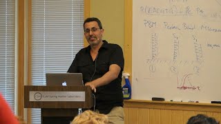
In this extended lecture, Adrian (with input from Rafael Irizarry) walks through the hidden sources of bias that plague high‑throughput gene‑expression experiments, from microarrays to RNA‑seq. He begins by illustrating how a naïve model with only 16 probes per gene can be stabilized by adding a small constant (e.g., 16 or 32) to avoid division by near‑zero values, a trick that dramatically reduces variance. He then shows real‑world cases where apparent biological signals (e.g., a quarter of genes differing between European and Asian blood samples) are actually driven by confounding batch effects such as sample collection dates. By examining PCA plots, correlation matrices, and timestamps embedded in microarray files, he demonstrates how hidden variables (year, month, reagent changes) can masquerade as biological differences. The talk proceeds to formal statistical modeling of batch effects, contrasting simple fixed‑effect adjustments with more sophisticated factor‑analysis‑based methods (SVA, RUV, COMBAT) that treat unwanted variation as latent variables. He explains why these methods sometimes fail and why Bayesian formulations are being explored. The second half focuses on RNA‑seq transcript‑level quantification. He describes the fundamental identifiability problem: reads often map to multiple isoforms, making direct estimation of isoform proportions impossible without a statistical model. He outlines the classic maximum‑likelihood / empirical‑Bayes framework (Cufflinks, RSEM, etc.) that links exon‑ and junction‑level counts to isoform abundances. Using data from the UVITAS project, he shows that even well‑established pipelines can produce thousands of spurious differentially‑expressed transcripts when batch effects are present (e.g., two labs processing the same samples). By drilling down to individual genes, he reveals how GC‑content bias in fragment generation leads to systematic under‑representation of high‑GC exons, causing isoform proportion estimates to flip. He introduces the Alpine algorithm, which fits a generalized linear model of fragment count versus GC content across the whole dataset to estimate per‑sample bias parameters, then corrects isoform quantification. Alpine dramatically improves concordance with ground‑truth data and mitigates batch‑induced artefacts. Overall, the lecture emphasizes a cycle of data exploration, hypothesis generation, statistical modeling, and validation, arguing that careful modeling of both known and hidden sources of variation is essential for reliable high‑throughput genomics.
Chapters
So, like you said, my name is Adrian. Here to give kind of a session on an introduction to RNA sequencing, but kind of up to when you see a paper or when someone describes results from RNA-seq. I kind of want to tell you about how the sausage was made up to that point before you actually started doing particularly sophisticated statistics or anything like this. So what I mean by this is when you actually do an RNA-seq experiment, your goal is generally to come up with some measure of gene expression. So the goal of this session is going to be kind of what are measured— like, what are the measures of gene expression that we can derive from RNA-seq? And what are our considerations to keep in mind? Where do they come from? And kind of what are the biases there? So I also want to make this like maximally interactive, so please interrupt me at any time during the session. So if we actually want to I want to start kind of with a map of what happens in the making of an RNA-seq sort of gene expression measure. And actually, this will also be kind of the guide for the talk. So we'll be going through the talk like this. So generally speaking, you're going to start with some kind of biological sample from which you will extract your RNA. You will then prepare a sequencing library. This sequencing library will itself go on a sequencer and generate reads, which you will then through a variety of ways come up with gene expression measure. And this arrow is actually a pretty fat arrow in that what it actually represents is any combination of tools that could include something like alignment, transcript quantification, quality filtering, taking care of a number of biases that arise at this point. And then once you have your gene expression measured, there's a lot of things you can do. There's kind of two sort of directions on this. Well, you might have had a hypothesis when you were doing your initial biological samples and that you might want to test something about that hypothesis. Maybe the gene expression changed in some genes between your samples. The other is you might not actually have a hypothesis. You just had a bet that there would be something that's different amongst this collection of samples and you're kind of going off in a sort of non-hypothesis guided exploration. Um, but the point of this talk will really be to try to get to this point and have a sense of everything that went into the making of that point. So hopefully these are all words that you've heard to some degree like sequencing library, sequencer reads, and so on. But never actually, or might not remember anymore the, like exactly how those were defined or where they come from. And the point of this talk will be to go up to that speed. Okay. Let's actually start with the biological sample and the RNA. So if you actually think in terms— when we say RNA-seq, what are we actually interested in? It turns out that it's actually a small fraction of RNA that we generally study. So if we actually look at RNA, most of it, anywhere between 80% to 90% will act in a given cell. And there's some variation. Based on the tissue, but also some variation based on whether you care on the kind of per-molecule basis or the per-nucleotide base. But 80% to 90% of this is actually ribosomal RNA, which encodes for ribosomes, which are used in translation, but not necessarily— we don't think of them as particularly dynamic or particularly easy to measure their dynamic changes.
RNA that's actually constituting the ribosome, or RNA that codes for the ribosome?
RNA that's actually constituting the ribosome, yes, ribosomal RNA. And another fraction of this 5 to 10% will be your tRNAs that are also necessary for ribosome function. And then finally, the actual part will be some 5 to 10% left that's actually the messenger RNA. And so how we actually Think of— so messenger RNA would be RNA that comes from gene— from expression of genes. And often they'll be protein coding. In the past, this would have been— I guess if they're messenger, they're actually translating a message, so they have to be protein coding. But we would now also— we could keep adding to this list things like long non-coding RNAs and many other classes of RNA that that have been discovered recently. The actual— so you might say, like, okay, so why are you starting there? Like, what's— yes, these exist. Why is that important? It turns out that when you're designing an experiment like this, one of the very first decisions you're doing is actually, how do I scope in to one of these classes of RNAs? Because you don't want to— it kind of comes down to a question of cost. You don't want to spend 90% of your sequencing dollars sequencing ribosomal RNA. So we try to bias our libraries towards mRNA. But in doing that biasing, we might— we start introducing kinds of other biases that we need to take into account and know that we're doing. So the two properties of mRNAs that actually allow us to enrich for them are generally twofold. One is you'll have a poly-A tail. On the 3' end. So this is not actually encoded in the genome. It's added by a nonspecific polymerase. And it can also have a 5' cap. And this cap— so there's a number of theological reasons why you might want to have sort of specific modifications on both ends so you can cells actually recognize that an RNA molecule that has those two on the end is not a fragment, but actually a full transcript. So we can kind of harness this to actually try to enrich for these RNA molecules. Yes, you're clear. [Speaker:AUDIENCE] Do I guess you could draw a picture of an mRNA and show what those things are? [Speaker:JOSHUA_ELKINGTON] Absolutely. So if we have an mRNA, this is a sequence of— RNA bases. On one end we have a poly-A tail, meaning literally a repeating sequence of A bases. And then here we have a modified— M5— we have a modified nucleotide on the very 5' end that's actually a cap that prevents degradation starting from this end. And this tail is thought to kind of behave as a buffer that if you start degrading this end before you actually start degrading the meaningful part of the RNA, you can degrade the poly(A) tail. Yes? How many As are there typically? Is it always the same? No, so it varies quite a bit. It's actually— so my perspective on it is how many As do you see in the data, as opposed to necessarily how many As are there biologically. I'm not actually sure the answer to that second question. This can vary from anywhere between 5 to 30 or 50, your main— the main issue is actually whether it was fragmented or not matters. And you will occasionally see in your data just stretches of continuous As. So how do we actually enrich for things that have this structure? Well, we could, if we're very, very careful, we can first of all do in our very— we can start a reaction that relies on having a poly(A) tail. Present. And we can also actually make sure we pull down things that have a 5' cap. Turns out that most sort of approaches would only actually focus on the poly(A) tail because it's easier to do. So we're taking this, which also means that we're likely to take any fragment that has a poly(A) tail, but unlikely to necessarily only have full-length transcripts. So, okay. So our goal is to actually do— so this is kind of— so if we start with RNA sequencing, this is the RNA in RNA-seq. Let's talk just briefly about the seq and then let's see how we connect them. What I guess the dash is between the two. So when we have— just gonna— So when we have sequencing, what we're generally referring to today, I think, when you say RNA-seq is actually Illumina-based sequencing by synthesis. So using the Illumina platform of libraries. You actually can do RNA-seq with the other technologies. I would just say kind of based on throughput and based on gigabytes of data that is available out there. Most of it is from Illumina sequencing. So what exactly is Illumina sequencing? So it's a method to actually get many, many short reads in a fairly cheap and very efficient manner. And so your input is a collection of double-stranded DNA molecules that have very specific sort of structure. In the middle, you actually have— your biological data or sequence that comes from some kind of mapping of your biological problem into a sequence. And on the extremities, on both ends, you have hardware that helps, that is necessary for the sequencing reaction to proceed. So let's actually talk a little bit about what this hardware is. And the reason for this is a lot of the Advances in a number of library prep methods that have come out in the last couple of years rely on actually sort of using this hardware more carefully. So this is a DNA molecule. Sorry, sir. So this is a DNA molecule. Its length could be anywhere between 200 to 1,000 bases. And what we have here are— We have something that we call— most externally we have something we call the flow cell binding adapters, generally called P5 and P7. Then we have— we can have indices. These are also actually sequences that you control that are used to multiplex, meaning combine several combine molecules that come from different samples onto the same sequencing run. [Speaker:AUDIENCE] Are those also known as barcodes?
[Speaker:JOSHUA ELKINGTON] Yes.
So indices— so the words you'll hear about are multiplexing, barcodes, indices, I5 or I7. When you hear this, you should think about this part of the sequence. And then finally here, you actually have another constant sequence that serves for priming of the actual sequencing primer. And so what actually happens, like how does this actually get sequenced? So if you've bumped into Illumina sequencing even a slight bit, you'll know that you should be expecting millions to hundreds of millions to billions of short reads. So what does that mean? So the output of the sequencing will be anywhere between 100 million to 10 billion reads. And so how do we actually generate this? So the trick is actually to take more or less a Sanger sequencing reaction that we've made more modern and can do in parallel on the glass slide. So yes?
So you said 100 million to 10 billion?
Yes.
OK. And are you going to come back to how we got from the RNA to the DNA?
Yes, I will come back. That'll be the dash that I'll get to in just a second. OK, so how do we actually do this? If we have— the way to start this begins— can people see if I write here? That's good. OK, so we start with a glass slide on which we actually have a lawn of two kinds of primers that are able to bind to these sequences— to these P5 and P7 sequences. So we actually have a lot of primers. And when we denature the sample and flow it over the flow cell, which is what we call this glass slide, these molecules are able to hybridize. And so this is actually great. We get kind of a random distribution of where these molecules fall on the glass slide. It should follow the density of how many molecules we get per surface area should be a function of our concentration and our hydration parameters, and we can play with those. And we could now kind of start doing a sequencing reaction. If we were able to actually see a single fluorophore being incorporated in this single chain of DNA, we could actually do the sequencing reaction on the spot without needing to do anything else. It turns out that actually being able to do that is very difficult. What's a lot easier is to actually locally amplify our molecule of DNA. And the way we do this is a process called bridge amplification, which is— or cluster generation, which is essentially doing PCR constrained with primers that are bound on a 2D surface. So what happens is we can then add a polymerase and bases which will extend this molecule. And now this molecule is bound to this glass slide. It's actually able to loop around and connect to a primer that might be nearby. And then that one can actually get extended as well. So after one cycle, you should actually have a double-stranded piece of DNA that's— both 5' ends are actually bound to glass. And you can keep repeating this process, and your cluster will grow in size based on kind of the maximum length that the molecule can reach. And you'll actually get along— all this region should now become molecules that share the same sequence up to the fact that they're complementary to each other. So you have two kinds of species that are complementary. And this actually, if you look from a kind of top-down perspective, where initially you had a single molecule landing, after this process of bridge amplification, You should now have a lawn of molecules that should all have the same sequence. You're then able to— you cleave off one of the molecules, one of the two species, just by having kind of a different chemical modification on the oligo that's on the flow cell, and then can actually start the sequencing reaction. So what that sequencing reaction is, is— so now imagine if we are here. And we are— so this is your 5' end. This is my 5' end. I am bound to this piece of glass. And I have removed, I have detached, and I'm only keeping kind of this strand of DNA. So I'm going to erase this. And now what I can do is I can bind a sequencing primer that's going to come bind right here. And I can start doing cycles of essentially Sanger sequencing, where I can try to incorporate various bases in these positions which have fluorophore bound to them. I can image which fluorophore got bound here. And the reason I can actually image this is not single molecule imaging, but it's actually the fact that there's a whole lot of molecules which are in the same stage of sequencing. So there's actually thousands of fluorophores there. Yes?
Sorry, just jumping back to amplification for a second.
So the cluster can just grow and grow and it's just the number of cycles that keeps it from spreading. Exactly. So the real sort of mastery between— the real mastery comes at being able to have it have the maximum density of clusters so that you can still resolve them independently. There's actually a number of things that go into that. One is actually just having hitting the right density even if each molecule were unique. The other thing is actually being able to resolve two molecules that might be neighbors but are similar. So if your sequence is very, very similar, you might start getting confused that a whole region is actually for some reason one cluster. So you want to avoid that. And then you would be careful and really not put that many molecules to begin with.
[Speaker:AUDIENCE] When you're doing the Sanger sequencing, I thought the bases were added from— bottom sort of up. Is that wrong, or did you just kind of draw wherever?
No, so your bases have to be added to your 3' end, so it just turns out that initially— initially, yeah, you actually— yes, you're heading in. Yeah, so pretty sure your 5' side is bound. It doesn't actually— I mean, you don't actually see that, right, because you're just seeing the top view, but I'm pretty sure that's the case. Okay, so now what actually happens— so what that actually— Sanger sequencing reaction is much more— it uses much, much sophisticated chemistry than Fritz Sanger had access to, meaning once you actually incorporate a base, it can't— you can't add on top of a base because the fluorophore itself prevents further polymerization. But you can actually remove this fluorophore and then keep adding. So that's how you're able to build on the same molecule while constantly imaging. And you keep going until something happens. So what actually happens? Why can't we sequence for a long distance? Turns out that your polymerase should actually be able to go with fairly high fidelity for a very long time. The only problem is because you actually have a cluster that's actually many, many thousands of molecules, If anything starts happening where there's a mistake in any subset of those molecules, the actual sequencing will now not be pure, meaning you're not sequencing the same sequence at the same time. So the actual signal that you get starts being a mixed signal that degrades over time. And this will be a function of how many— if at every cycle for every molecule in your cluster there is a chance of incorporating an error, this will grow as you're sequencing. As this length grows. So this is how we sequence this first read. And then what we can do is we can actually just remove this part. We can actually have this bind to— so actually we can then bind a second sequencing primer, which is not read 2, but the complement of read 2, which would bind here, and we can read our index. We can then have this do one cycle of bridge amplifications to do like strand flipping, meaning we'll now have this bind to the primer that's still there and grow out the reverse complement now bound like this. And then we can repeat this cycle now actually reading into here and then reading this thing. Okay, so now the drawing is actually a little bit messy. So let's summarize what actually did we read for every molecule. So we got read 1. Which was some sequence as far as we could go, or some sequence that could be anywhere between, say, 30 to 200 base pairs. We got— this was primed by this primer. We got read 2, which was also reading into the same segment of biology that was also anywhere between 30 to 200. And then by using the reverse complements of those reads, we're actually able to get the indices. Which we call I5 and I7. And these could be anywhere between 5 to 8 base pairs. They can also get longer. This is kind of the current standard. Yes? Excuse me?
Why do we need them?
Why do we need the index reads? OK, so the reason we need the index reads is if I'm doing an experiment and I have 10 samples, And based on my experience, I know that if I get 10 million reads from each one of my 10 samples, that's good enough for me. So that would actually mean it's 100 million. I need 100 million reads for my experiment. So now there's two things that could happen. I could either just sequence— and let's say I do. So I use a machine, say the NextSeq 500, and I use it on settings that would generally generate somewhere between 400 million to 600 million depending on kind of that clustering density that came up earlier. So I might actually have more reads. I can't have the machine do— it uses the same amount of reagents, it's the same cost, so there's no reason for me to try to make fewer clusters. I can either use that extra data, great, or I could actually try to see if anyone else in the lab, or if I have a different experiment that I could combine on that same sequencing plate. And so the way you would combine this data is by saying like, okay, so when I do my library prep, which I'll explain in in 2 minutes. I will incorporate— when I make my 10 samples, I will incorporate a different index for each sample here. And maybe this— and maybe this— [Speaker:AUDIENCE] To distinguish between samples. [Speaker:PROFESSOR] Exactly. So to distinguish between samples. And the way you do that distinguishing is just in silico. After you do the data analysis, you identify them based on the barcodes. Yes? [Speaker:AUDIENCE] If you're going to sequence once and then do pre-amplification and sequence from the other end, why do you need to also stick a primer a separate primer to get the index towards the 5' end. So why not just sequence through this read, or what do you mean? I guess what I'm wondering is the primers you actually use for the sequencing, are those going to be the P5 and the P7, or are those just— No, the primers are— P5 and P7 are what you use to be able to bind to the full cell. And so why? Yeah. I think I understand. Why isn't the index just on the other side of R1 and R2 so you can get the index? Oh, why it's in here? Why isn't the index essentially the first part of your biological sequence? Yeah, that's a really good question. It turns out the reason for that is because— so it's actually a lot easier. It makes the addressing easier to do. And the reason for this is I'll get to in just a second as we talk about library prep. The point is that this allows you to add the index as kind of a last step of PCR as opposed to having to design kind of your entire strategy around it. So you could build an entire library prep method that is completely agnostic to how you're going to add the indices, and at the very end you get to add your indices.
Yeah.
Okay, so that's how sequencing works, and I'm going to need to erase a bit. And let's actually— so how do we actually get this molecule? Right? So let me redraw it. Wow, you weren't kidding. Okay. We'll avoid doing that in the future.
Okay.
Will that help? Seems like desperate measures. Okay. We'll let it dry. OK, so how do we actually— so our library, like I said— I guess I'm tall, so I can do this. Our library is a double-stranded molecule where this came from our biological problem. We had this be our indices, and then the rest are sequences that came from Illumina. So how do we actually go from RNA to something like this? So this is the process that— this is what we refer to when we say library prep. It turns out there's many, many different ways of doing library prep, of mapping from this to this. And actually, they'll actually introduce completely different biases. I want to show you an example of one that I think is simpler and also has several of the features, several of the most more advanced features of the more modern library prep methods. Okay, so how does this happen? So we have our transcript conveniently placed right here. And what we're going to do is we have an RNA molecule. We can use an RNA-dependent DNA polymerase that is primed with a poly(T) primer and can transcribe starting from the primer can polymerize and make a fragment. So where we have an RNA molecule, we now have a DNA molecule. So we have an RNA-DNA duplex. And again, this is just one way of doing it. There are many variations, but this is one that I think is particularly clear. Okay, so we have our— DNA-RNA duplex. We now need to somehow get to it. Most enzymes can't actually work with DNA-RNA duplexes. We actually need to make a DNA-DNA duplex. And so this is called— so this very first step was RT. To make the DNA-DNA duplex, we're actually going to do something called second strand synthesis.
Yes?
So these are a— this is a DNA primer that you're supplying. And yes, reverse transcription. Yes, that's what RT stands for. Thank you. So let's expand out reverse. And this is second strand.
Synthesis.
I would say this is the actual dirtier secret in the lab is if you actually want to have fun with someone who does this very, very routinely, go like, how exactly do you do second strand synthesis? And it turns out it's generally a proprietary mix of enzymes so that since at some point in the 2000s, people have stopped knowing exactly how it's necessarily done in your mixture. There's a variety of tricks you can do. One, and the kind of the main question is it depends on how much you care about really getting this very end of your transcript. Right, so you can do something that's called strand inversion where you have a kind of nonspecific priming that can happen. So your reverse transcriptase might have the property that it often adds a triplet, a nonspecific triplet of GGGs at the end. And you can use this to prime the synthesis on the other side. Or you can use any number of methods that were developed in the '80s and '90s where you can introduce nicks into your RNA and then use the same reverse transcriptase to actually kind of fill in your DNA molecule. But in both of these contexts, except if you do this priming based on this nonspecific triplet, most of these will— you'll start chewing back at this 5' end. So actually here, we have no guarantee that our reverse transcriptase will will synthesize all the way into the end of our molecule.
What lengths are you— how long are these molecules and how far can you get to?
So these molecules— so the starting molecules are mRNA transcripts. So they vary enormously in size, right? We have very, very short transcripts that can even be coding on the order of a couple hundred base pairs. And then we have things that are like 10 KB. And your distribution of— you'll generally be, again, introducing a bias for shorter things. So maybe we should actually keep a tracker of biases. So shorter things. And this came at least— this will come in many, many steps, but it comes at least in the RT step. And we also lose the 5' end. This will happen in RT. It will also happen in second strand synthesis. Yes? I'm sorry, there's like a row. Yes, you. At this point, does the sum of the transcripts have introns in it still, or are they spliced out? At this point, we expect most introns— our assumption is that introns are spliced out. So if you actually need them not to be spliced out, you need to isolate the nucleus because that's the only place where these pre-mRNAs exist. And you need to try— and there's, I guess, enrichment methods that you can do to try to pull down things that are in the process of being spliced. And the issue there is we often think of transcription happening and then splicing, but that's not actually true, right? Especially for very large transcripts, there's evidence that splicing can happen kind of in the process of transcription. And so actually getting to— so I'm assuming That you have spliced, like mature mRNAs, yes, which would mean have been spliced. Yes, there was another question.
Sorry, what's the source of the first bias for shorter transcripts?
So this is, you can think about it as the time it takes to actually prime, to actually do a 10k. The probability of any, like a falloff event, if you think about the probability of anything bad happening, let's just be general. Would scale with every base pair that you incorporate in reverse transcription. So the longer— and you're talking like a 10 or 15 KB transcript— you have a much higher chance of something bad happening for that than a shorter one that's like 1 KB. And that just kills the whole molecule? You'll have a fragment that will— so maybe you either lose the whole molecule in some way, or more likely, you start clipping that 5' end in a way that's length dependent, as opposed to just, oh, You just ignore all 5 primers. Yes? You don't actually need that many bases after the poly(A)-tail if you just want to align it and figure out which gene it is. We'll talk about that. It's just the splice form that you care about. Exactly. I'll try to get that at the very end. Yeah. OK, so we have this. We make this molecule. We make the duplex. Now what do we do? So the actual thing is we have— there's a lot of information in which strand we're on. So this is an asymmetric molecule. If we made the duplex sort of— illy-nilly, we'd actually now make a symmetric molecule, and we wouldn't know which part was originally in the 5' and which part was in the 3' end of the molecule. So what we're actually going to do is we're going to add uracil bases into this DNA synthesis reaction. So where this strand did not have uracil, when we make the next one, it will. This will come in handy in just a second. So now we've got this synthesis that happened. Okay, so again, this is just one protocol of many. But we're going to add a polymerase that is nonspecific, that is able to add just a single A base pair on both ends.
So when you say add uracil, that's still DNA?
It's DNA, just made with DNA uracil bases, which we can synthesize. You wouldn't really see these in nature, but we can synthesize them chemically. You don't see them in nature, but they're the result of mutation. And that's actually why we'll have a very helpful enzyme in just one second. Okay, so we now have this molecule that is not a perfect duplex but has a one base overhang, which we can actually use to ligate in a fancy adapter, which has this shape. It's a hairpin loop where in the middle there's another one of these mysterious uracil bases, and then we have And we can ligate— so we have both of these. And the important thing is that this adapter is not symmetric. So on the side that binds to the A, we can have either the P5. We can actually— this barcode is what incorporates this part of the hardware. So this is not symmetric, so this will either have the P5 on this side, which would put P5s here and P7s here, or the opposite, up to you. Okay. So why did we incorporate those uracil bases? It turns out there's enzymes that remove uracil bases in DNA. So we can add this enzyme, which will now actually excise out these uracil molecules. So what do we end up with once we do that? We end up with one nice piece of DNA that is the reverse complement of our starting material, that has P5 on one end and P7 on the other end. In fact, has the whole Actually, in this case, let's say it has just— you only add in this fragment for now, R1 and R2. You'll see why I'm making this change. So you're doing this, and you have these fragments, which you can actually wash off and degrade away. So the only full-length molecule— so you can either wash them off or degrade them, or what you can do is you can prime a PCR using R1 and R2. And these fragments don't have a contiguous R1-R2 sequence, so they'll just be degraded. And this will actually allow you to remember that when you sequence either R1 or R2, you'll be able to map back out to whether you're on the positive strand or the negative strand. And that can be very, very helpful in your downstream analysis. If you are going to do PCR, then does that go to bias? Yes, exactly. I'm adding that in just a second. OK, so now we have a molecule. So I've done this for each one of my samples. I can now add different primers. That will bind on R1 but have potentially different indices for different samples of mine or different samples from collaborators. And then I can do PCR. So this was deamination, which you can think of as removal of U. And then we can do PCR to amplify our library. And then we can stick this on the sequencer. And we've never at any point— so if you didn't do this step with the uracils, you would actually not know which orientation things came from. You would have P5s and P7s on both sides because both of these molecules would be able to prime PCR. And then you would have a non-strand-specific library. So we added PCR. What kinds of biases would PCR introduce? So the main— so again, it might enrich for shorter things preferentially because they could— they'll have a higher probability of amplifying. But you might also start introducing sequence-specific bias from the PCR. Okay. So this is actually kind of nice where I'm writing like one bias comes from this step in library prep. But you should actually notice that, well, we introduced sort of the mother of all sequence-specific biases when we primed with poly(A). Turns out we like to think that all mRNA molecules have poly(A) tails. That's not true. In fact, many long non-coding RNAs don't have poly(A) tails. So this also, you know, the poly(A) selection also introduced a very specific kind of bias. But this bias is different because if the reason— what this bias will do is it will actually start changing the composition of our sample. So molecules that more readily amplify will have a higher amplification efficiency, meaning on every cycle in a very, like, really, really good molecule, every cycle might actually give us 1.9 times the number of molecules we had originally. One that doesn't amplify so well, we might get something like 1.6 or 1.7. But when we repeatedly exponentiate that number, the difference between the 1.9 to the 20 and the 1.6 to the 20 is pretty large. And we'll end up with having enriched for a specific kind of transcript. Now hopefully all of these biases are consistent across samples.
Maybe.
Or they're not. And that's something you have to keep in mind.
OK, great.
So what do we actually do with all of— so we had a biological sample. We had RNA. We made a library. We then stuck this on the sequencer, and we got hundreds of millions of reads. And using the indices, we were able to map out, or we were able to figure out which sample each of these reads came from. And so what do we actually do? So there's kind of the standard approach, which was kind of true for many— let's say the first 5 years of RNA-seq. And then essentially people were like, ugh, this is slow. We could even be more precise. And then people came up with more modern methods in the last couple of years that I'll briefly mention. But the simplest version of this is you take your read, and our assumption is it should be coming from the genome of whatever organism we're sequencing because it came from an RNA molecule that was made from that genome. So let's just align— so what do we do in the analysis? So we can just align the genome. And so where we started off with just a collection of reads, we now have a collection of reads with some metadata about which location of the genome do they match to. Hopefully just one, but maybe several. So this was our alignment. This will actually produce SAM or BAM files. Again, maybe extensions you've bumped into. Whereas the raw reads were FASTQ. OK. Before we actually do this alignment, we might want to throw out reads that are bad. What does this mean? This means whenever— the FASTQ is actually not just the sequence of the read, but also an assessment of the confidence of the base call during the sequencing. So you can actually say, okay, if there's a stretch— if I take a read and there starts being— the quality across that read is low, I might want to just get rid of it all, or I might want to trim it back. So we have this alignment onto the genome with those reads that we felt were confident. Where we felt were high quality. And then we can then take a reference transcriptome and see how many reads map to a specific gene. And for now, let's actually not try to distinguish between different transcripts. So if I have a gene and I have exons and I've got reads that map here, I might say there are 5 genes— 5 reads for this exon, 5 reads for this exon, and then I have another gene that might have a single read. OK, and now we need to come up with— that could be an expression measure, right? We could say in my sample for gene A, I had 10 reads. And for gene B, I had 1 read. Often we'll call these counts. So how many counts did you see? So except if you are very, very lucky, you will have gotten a different number of reads for each one of your samples when you go on to the sequencer. They'll probably be close, but you'll have gotten a different number of them. So if you had 10 times as many reads for gene— for sample— for Let's actually make it— so this is sample 1, and then this will be A and B in sample 2. And here maybe we had 2 and 0. So these numbers are very different, but of course this could just be because you had 5 times as many reads on this sample than on that sample.
You started with more material from that sample?
It could be that you started with more material. It could just be that you accident— that you— you had something happen in one of your PCRs. So it doesn't actually map back to a biology interpretation necessarily. Or it could be that when you actually— so the way this actually works in practice is you make your libraries, quantify them independently, and then try to mix them in as close of a ratio as possible. But it can be shockingly hard because of differences in size distribution.
And every sample has to have its own library to have its own barcodes?
Yes. And you can actually choose to put several barcodes for the same sample. To be able to estimate any effect that might come from your barcodes, or to increase the diversity of the library. OK, so we can come up with this number, which are counts. We can then just divide this by the total number of reads that came from that library to make something called counts per million. And that's a very useful metric, but what's missing is we're not accounting for the fact that gene A, for instance, might be long. We can now compare between A and A and B and B between our different samples.. But we can compare genes within the same sample. And the way we're gonna do this is we're gonna normalize to make an RPKM or FPKM, which will actually be a normalization based on the length, the total length of our gene. And so that number is— The way we would write it out— so if CPM was counts divided by R, where R stands for your library size, this would be— and let's actually have counts be RG. This will be RG divided by the length of the gene itself divided by 1,000. All of this over a million. What this stands for is reads per kilobase of exon model per million reads.
Yes?
So RG equals counts over R? Yes, RG is counts. No, CPM would be RG over R. And yes, you're right. My R is missing. There would be an R right here.
Thank you. So when you say library size, you mean The number of reads.
That's— okay. That's what I mean. Um, it turns out that that's not actually an accurate— the number you should be using for R. And the read—
okay.
So finally, this has a cool prop— this is useful, but a property it doesn't have is that it doesn't sum to the same number. This might be a property that you want. So if you just take the sum of all your RPKMs, different samples will have different RPKMs.
The RPKM was pretty fast.
Can you go through that one more time? Um, so okay. So what do we want to normalize for? We want to normalize for the number of reads we had for our sample. That's easy. We just divide the counts, RG, by the number of reads we have. But our expectation is actually that every position along a gene has an equal probability of producing a read there, which means that a longer gene has more opportunity to make reads than a shorter one, and it should make more reads.
[Speaker:AUDIENCE] So can you explain that?
If there's one poly-A tail in an RNA regardless of length, so why is the longer— Right. So, yeah, you're right. So when you actually— so there is a step at some point, which I should have been looking at my notes that I skipped in this library prep protocol, where at some point you will actually introduce a— in this library prep protocol, you actually might So let's actually see how you would do this in this library, in pyprotocol, is you will have a step where you randomly fragment your DNA to produce opportunities for reads along the whole length of your read, as opposed to just your 5' end. The way I've described this, you would only actually ever sequence one end of your transcript, and you would actually get every count being one molecule. But yes, so you can add in a step where you randomly fragment your library and then amplify on one side there. And then take this and bring it into your PCR reaction.
Right, but you have to—
the primers can go back on the pieces. Yes, so the way you would do that, so you would actually— you could do your fragmentation when you had your one molecule. And then you can actually ligate in specific adapters, like do a nonspecific ligation. Onto one end and then use this to prime your reaction. Similarly to how you had the loops. Exactly, yeah. So you could do— it's actually a different enzymatic reaction, but you could have something that's specific to the 3' end. You can have something that's physically the 5' end. And you can add site-specific primers. So this way you can go into the interior of the molecule.
Exactly.
But also the number of molecules in the library that you get will be— [INAUDIBLE] Exactly. And then if you're doing this— and thank you for that— if you're doing this, then you actually need to normalize for your length of your gene as well.
And the indices are somehow retained when you're—
So the indices would still happen. So if you were doing this kind of process where you fragment and then randomly ligate something, again, the only thing you'd be adding in would be the R1 and the R2s. And your indices would be added in your following step of PCR.
Yeah. So this is like Nextera?
Is that the— This, I know for a fact this is NEBNext, like the New England BioLabs one. I'm not actually— there's many versions of Nextera actually, so I'm not sure exactly what it maps to for that.
Okay.
So we can come up with this measure. I just want to define one last thing, and this one's important because its name would make you think it's something that it's not necessarily, which is transcripts per million. Which is you might want the property that all of your samples I'll get to that in just one second. Have the same sum to the same number. And the way you would do this is you would actually take your reads over your lengths times a million and divide that by your sum over i of your number of counts divided by your number of lengths. So this will sum to 1, which is, could be close to an interpretation in terms of fraction of RNA. And it's called transcripts per million TPM. But it doesn't actually mean that you necessarily, in this way, if you've done the analysis this way, you've not actually ever at some point quantified specific transcripts. Okay, I want to take 3 more minutes to kind of just mention a few words that you will bump into that I think are particularly important. So it turns out that this way of doing it, I think, is the, you know, you align, you count, is kind of the old school way of doing it. It turns out that if— and it actually— you might have noticed that I at no point— I just said the length of the gene is the total length of the exon models. I at no point made a difference between different transcripts that might come from the same gene. And so what actually happens there is if you need to account for transcript abundance, you can do something called expectation maximization, EM.— to actually try to quantify the problem. If I have several transcripts that have— that use different exons, for instance, I might have— this might be my gene, but I have one transcript that uses these two exons and then another that uses these two exons. And you see where reads map, you can actually use expectation maximization to actually try to estimate the relative ratio of these two RNA species. So that was how people started doing differential expression between splicing isoforms. And then people realized, wait a minute, we could actually do EM in a— forget alignment, we'll just do EM on short snippets of our transcriptome and short snippets of our reads. This is called a method called Sailfish, which turned out to be super, super fast because you skip aligning, which is slow, and actually quite surprisingly accurate. And then people pushed that idea further being frigate tamers. Forget just K-Mers, we can actually simplify down K-Mers to a class of K-Mers that have a property based on— that have a shared property and we can do expectation maximization on that. And that makes this process take anywhere from literally days of computations with something like TopHat2 to 10 minutes with a tool called Calisto. So I will write them down here. And it's Kalista with a K. And then I think two else. Is there a good review on the, the little story you just told of the different, the different ways you could, uh, well, the, the, yes. So I would actually just go to both of the, the papers are pretty new. Yeah. And they're very— just Google these two names, um, then there probably might be a review out at this point. Start with the same. OK. And OK, so we've got this. Two things I want to mention. People have started going really, really crazy on what they actually include in these sequences and how they bring in— like what information they put in your indices. One of the best, coolest tricks that came out recently that I want to mention, and this will be the last thing that I talk about, is unique molecular identifiers. What this means is if when we start this reaction we actually include behind the poly(A) tail a sequence of random bases, and then maybe a handle so we can do PCR with this, we will be able to do something very, very useful, which I'll explain in a second. So we can then prime a reaction, and maybe we don't actually do fragmentation. We do a fragmentation step, but only select things that have this handle. And then some random piece of biology on this end. So instead of kind of just dealing with the fact that we have some 5' bias, we can actually completely give up the 5' end of the molecule to retain a fragment here and a unique molecular identifier. And then proceed through sequencing, and you can sequence this fragment and this fragment. And now your expectation— the reason you do this is you want to be able to distinguish several original copies of mRNA that had the same sequence from PCR duplicates. What this means is if when you actually do your analysis you notice that you have a gene that generates many, many reads here, but they always have the same sequence of bases pairs here, that's very unlikely to have come from the fact that you had the same primer always binding. It's much more likely to just have been one molecule that bound and created this, and that got amplified 6 times. 6 times. If instead you see 6 molecules here that have the same sequence but have different barcodes, you know that they came from different original molecules. And that's an incredibly helpful method in terms of being able to distinguish this computationally and try to solve some of these bias problems. These are called unique molecular identifiers. Then people said they're not unique, so people started calling them random molecular tags. But this is what— whatever you refer to. OK, I want to end here so you guys have time for everything else.
Looks like you're still setting up for a moment.
So if there are any questions at this point— kind of had to rush through that. Yes?
Back to the question of introns, to the extent that you do have some reads. Yes. With introns, usually you think of you're only counting reads from the exons.
Wouldn't the—
if you're not interested in and didn't transfer to only how many quantifying per gene, wouldn't the intronic reads be useful?
So, okay, so you do actually have intronic reads. You also— so what pathologies arise when you align? So one is you could have intronic reads, but you could also have reads that came from a different gene that sort of accidentally mapped to your gene. So one way to try to minimize the effect of these sort of bad mapping events is to look only in regions that we know are particularly clean, and this might mean excluding introns. That's actually a decision you get to do when you say— when you say, how do you define your counts? Do you mean anything that maps from, you know, a start of transcription to an end of transcription including introns or excluding introns? And that's actually a decision you get to do. I would say 98% of the papers blindly excluded introns read and never actually looked at them and might have missed out on a nonspecific— sorry, maybe on an intron inclusion event that they didn't expect. Does that kind of answer your question?
So you're saying that often things map more uniquely to exons?
Yeah, so if you actually look at where your reads map, you could discover exons based on the fact that you'll have a lot of reads mapping in that location. But you'll often have just a smattering of reads that are intronic. Generally speaking, people just ignore them. But then there's actually papers where the whole point of the biology was an intron was retained, and that's what's causing your biological phenotype, and you might have missed that.
Yes? So if you're interested in transcript quantification— Yes. So say you put in this random molecular Yes. You also do this PCR amplification at some point, right?
Yes.
So with that PCR amplification, don't you turn a risk that you are amplifying your UMI many times, so you end up sequencing a lot of the same?
Yes, it's actually very disappointing. The moment you add unique molecular tags, you then realize that, like, damn it, I'm sequencing the same molecules over and over again, like a lot. What you actually do there is you can come up with an expectation for if I had this many initial molecules, and assuming my barcodes are well distributed, what distribution of UMIs should— like what's the mapping between number of UMIs that were detected for a gene and original starting molecules? And you can try to solve this problem back that way.
Yeah.
All right. I'm still around for questions.
Perfect.
Lights get ready and then we want to get everyone back in here fairly quickly and start the next talk soon.
Thank you so much, that was awesome. I started teaching statistics to biologists, computational biologists, a long time ago and originally the class was meant for statisticians but I The only people who would show up were biologists. And I noticed that they were being not necessarily forced, but they were just becoming data analysts, not always by choice. And they had nowhere to learn. They already finished. They had a PhD. It was hard to go back to school. So I decided to make this course with that in mind. There's a lot of people that want to learn this and realize they need to learn it after they're done with school. So it's a way to learn it at your own pace and without actually going to a physical classroom. So they're offered via edX. And you go at your own pace. You can actually get a certificate if you want, although that's totally optional. And there's quizzes where you learn to use R to analyze data. And there's a discussion forum, people, you can get help there, etc. So it's, that's the resource that he was talking about. Okay, so today what I want to do is just tell it, talk a little bit about some of the research I've done in the past that relates to the title of the talk. I'm going to end with RNA-seq, but I'm going to start with other technologies, just to give you a sense of what I mean by overcoming bias and batch effects. So to motivate the talk, I like to open with this example. This is an out-of-focus microscope, and the point— the reason I put it up is because the— there's a story, part of the story of science is that the person Antonie van Leeuwenhoek, who discovered microorganisms— he's considered the father of microbiology— wasn't considered like one of the top scientists at the time. Like Locke was around, I think, at that time, and he basically improved the microscope. So while other scientists were looking at pictures like this, you could actually see what was there. So the reason I like to start my talk with this is because I feel like that's what the job of the data analyst in biology is today, where the data comes in, you know, out of focus, and you can't— there's no biological insights to be gained out of noisy data. Once you put it into focus, then your collaborator or yourself, if you're the biologist as well, can actually make a discovery. And of course, it's much more complicated complex in the microscope because it starts out as digital data, so it's not even light that you're looking at. So with that said, I also like to show these Tookie quotes that have to do with exploration, with data exploration. I'm trying to make this point as much as I can because I'm seeing a movement in science to be more industrial in terms of just getting pipeline done and just having it ready and you see that, you know, go to talks and you see the little PowerPoint cylinders with the little square and the arrows, right, and at the end there's knowledge. So what I want to do is push back a little bit on that because I think those arrows, there has to be humans in there sometimes to think about if this is right and also explore the data, look at the data to make sure that there's no problems. So I'm going to give you some examples of cases where exploration of the data led to data analysis insights that then improved the data and then led to biological discoveries. So I can give you more examples. I'm just going to go through a few. I'm going to start with my first one where I was perhaps when you're at your level in your careers, as many of you. So this is in 2000, early 1999-2000, we first get microarray data. And this plot— this is the actual data, it's not an illustration or a cartoon— is showing you a PCA plot of gene expression measurements from 5 different tissues. And we have various replicates for each one. So you take the vector of gene expression, which in this case I think is a 12,000-dimensional data point. And what PCA does is it approximates the distance between these very high-dimensional points with 2 dimensions. Sometimes the approximations are very good, sometimes they're okay, sometimes they're not that good. In this case, I think it works pretty well. So you have 2 dimensions, 1 and 2, representing— and then the distance, the actual distance that you can use a ruler to measure, is supposed to be related to the actual distance between the measurements. All right, so those are the points that you see when you take the original data, which I want to call out-of-focus data. You put it— you just do a PCA, and if we didn't know that gene expression was different between tissues and similar within tissues, we look at this picture, it's not very revealing. Here are the actual tissues. There's some grouping, but it's not great. So you can see, for example, that placenta is closer to colon here, and then this colon is closer to— I'm sorry, this is endometrium— but this colon is closer to this placenta, even much, much closer than that one. That doesn't make much sense. So that was data out of focus. Okay, so this was put through the pipeline, the standard pipeline at the time, which is very young. But it was a standard pipeline. Papers were being published. Many papers were being published with that pipeline. So we wanted to know, why is this? Why is this looking so bad? Is the technology not good? Have biologists been telling us incorrect information about gene expression in tissues? What's going on? So this is where the first instance of looking at data comes in. So we went— this is actually a good example of looking at data at a high level, we went down to a lower level, look at 2 points, take 2 of those points and just look at all the data points for that. So instead of just 1, 2 dimensions, let's plot them all. So here are all the 12,000 points for 2 of those points, original points. Now this is actually from an— this is actually not from that plot. It is gene expression from microarrays but it's from an experiment we ran where we put the same material, or stochastically the same material, so we take— we split RNA sample into two. We put it on two arrays and then we compute the log ratio. We compute the average log expression. So genes that are highly expressed are over there, low expression on here, differentially expressed are here and here. This one's 16 times bigger This log base 2, 16 times bigger on one sample compared to the other. So this is supposed to be the same measurement twice, but it's clearly showing measurements that aren't in agreement with that. The experiment also included 16 artificially included transcripts. Those are the orange ones. Those are supposed to be different. All the other ones are supposed to be the same. So in a perfect world, you would see a line of all the black points on 0, no difference, and all the orange points at 1, the difference. But that's not nearly close. You actually have thousands of points with full changes bigger than 1— bigger than 2, sorry. I remember at the early days, that was how you defined differential expression. If 14 is bigger than 2, it's differentially expressed. It's clearly not the case. So now, so we see this plot and we ask, what is going on? Why is it so noisy? And the noise seems to be much bigger for the low expression values. Now this is a plot. This is an MA plot, for those that know what that is. It's now used all the time. Back when we started, it was kind of a new thing. Although it was already— if you go back in the literature, there's something called an Altman plot that is the same thing. That goes back, I don't know, to the '60s. Okay, so why is that happening? Is it that the microarrays don't work? Is it just that biology is somehow like that? But it can't be biology because we actually just split the sample random. All right, so now what this inspires is once we see this problem, then we ask ourselves, can it get better? And can it get better? Which— can it get better by improving the protocol? That's one possibility, which we really can only provide plots like this so they can then say, oh, maybe it's this, maybe it's that. Or is there something statistical we can do to make it better? So that's something that we struggle with whenever we encounter a new technology. Is there something we can fix, or is it something that the experimental biologists need to fix, or is it a combination? So this is kind of the world that I live in. I'm always finding problems and telling the experimentalist to fix something, and then we keep going, and eventually we converge on something that hopefully is better. So in this case, one of the things we realized is that before you even get to these points— this is one measurement per gene and then two samples— was that there was all this statistics that was done before you even got to that point. So this was in Appendix D in the manual of the Affymetrix company sent with their scanners. And what they did was they explained that each measurement had— came from 16 separate probes, and each one had a background level that needed to get fixed, and this is how they fixed it. So here's a statistical model that they were in a way thinking about. So you had the measurement of gene expression. We're trying to get to beta. That's the actual value, that's the value they want to measure, but unfortunately for them there was this alpha. It was this other background level, has to do with cross hybridization and other things that needed to be fixed. So what they did was they added another measurement, so they took half of their chip just to measure the background level. And then the hope was that once you have the background, one of the probes measures the background, you subtract them, And you're set. And you're ready to go because you have now what you want, which is the beta. OK, now two things. We care about log ratios, so we're going to take the log of that eventually. And we usually— and yeah, we care about a ratio, and we usually take the log. So we did another experiment just to get an idea of how correct this model was. And this is an experiment where we just created an experiment where it's all background. There's no beta. So in this experiment, now I'm plotting Y versus Y2. So there's— every probe gets a point, and you can see that there is in fact a very strong correlation. So they're doing something right. And there's also something that explains why they needed that, because every probe had a different background level. Look at the range from 4 to 12 in the log scale. That's 100— more than 100-fold. So this is all background. So background can be that— varies that widely. But the one concerning thing about this picture is that there's noise. It's not on the line. So this model is wrong. It's deterministic and the data shows it's not even close to being deterministic. Instead, it's something more like this where you have background levels that are correlated. Right now I'm saying they're not the same, they're correlated. And that change is— that actually has a consequence, mathematical consequence. You can show this, that the variance of the log of that correction they were doing— this is like Taylor's theorem, it's like a simple mathematical derivation— is going to be proportional to 1 over— that should be a beta, maybe signal beta squared. So that's saying the smaller the beta, the bigger the variance. That's a mathematical fact. It's not biology. It's mathematics. So here you can actually see that. If you think of variance as this, you can see the 1 over beta squared. This is an estimate of beta. And you can see it going up. So it's actually pretty— now in hindsight, it's actually pretty simple and straightforward that that would happen. So what we did instead is we used statistical ideas that estimates beta without the— estimates beta known under this model. And when you do that, now you're minimizing what's called mean squared error. So you're not going to permit a solution like that that increases the variance in that way. It just happens. The mathematics just make it happen. So when we started with this and after our correction, you then got this instead. So this is not a new experiment, same data, it's processed differently. And now you can see the noise is reduced and these guys stay up and it's much better. And now we go back to this picture, so this is data out of focus. Once you process it with this new algorithm, this new statistical approach, it turns into that. And now you can see the tissues. All right. So now you can make your discovery. Of course, we know this already, but had we not known it, we wouldn't have discovered it. With this microscope in focus, now you see that, yeah, tissues cluster when you look at the next patient. So that's my first example, just to give you an idea of what I mean by looking at data exploration, and then that motivates improved methods for improving the quality of the measurements you use for your for the biology that you consider important. Yeah. So the difference is— so each point here is the same gene measured twice. Yeah, right. And so in each case you have a Y1 and a Y2. And don't— but don't get confused with those Ys and Y2s. No, you're not talking about— it's not that. It's not these two. This is background and signal.
Right.
For each of the two, you split the sample in half.
Yeah.
And you have a Y1, Y2 for sample A and Y1, Y2 for sample B. Yeah. For each gene. And the only difference between this plot and the next plot you're saying is that you basically have— I mean, you're doing an expectation under a model that Assumes greater variance in lower counts through this log. That's the main difference. And—
but—
I'm still— it's still very surprising that it makes— like, you just have these 4 numbers. It's not just 4. Yeah, okay. So where does the power— where does the power and order going into it to make it that—
because you're doing the surround thing too.
It's more than that. So first is 16, not 1. Each gene has 16. But the other thing— this is a very good observation— 16 probes. That's not nearly enough. It's not nearly enough. You're right in asking that. Where does all this power come from? Yeah, so I skipped that, but good observation. So when we model this, now we're saying that these things follow some distribution. How do we know what distribution that is? That's where we use all the data in the— It's empirical-based. And that gives you— That together with having 16 probes. But I'm also going to say, in hindsight, this is actually quite simple. So if you were in a hurry and you wanted to fix this, all you have to do is add a constant, and a lot of these gains are achieved. That's something that once you think about it, you say, wait a minute, I could have just added a 32 in, and you almost achieve this. But adding the constant is sort of regressing What would mean? It's the concept being that when you have— when you're dividing by a small number that's random, the variance goes way up. But if you keep that number from getting close to 0, it doesn't happen. So even with RNA-seq, if you have an RNA-seq experiment, you see like all this noise and you're in a hurry, add 32, add 16. And then you can cite my paper. Adding 16 solves everything. Okay, yeah, it's a very good observation. Yeah, no, it's true because it's one of the things that we do is we want to have like a good reason to do these things too. We just don't want to do it because it worked once. So then by having a model, it just makes you feel more confident that what you're doing is the right thing to do. But sometimes ultimately there's a solution that's super simple and then you get made fun of for all your fancy math when all you had to do was a simple thing. Okay, so now I'm going to move on to— let's say we fix that problem, we think we know how to normalize data and get it preprocessed right. In this gene expression— I'm still with gene expression and microarrays— this is another good example, I think, of the power of always looking at data and thinking about, does this make sense? So this is a paper that came out in Nature Genetics, and I don't want to single anybody out, but it's a very good example and I want to use it. So here's in the abstract it says this. So they're looking at gene expression in blood and then they make this very, very surprising— they have this very, very surprising result. So one quarter of the genes tested are differentially expressed. One quarter when you're comparing blood from Europeans and blood from Asians. All right. Well, that's very, very surprising. And— but, okay, so when you see something like this, I mean, I wonder if there's something else and going on. So here's a plot, again, a PCA plot. And by the way, if you go through the pipeline, you do get that result. If you just go to the standard pipeline, Normalize your data, do a t-test, p-value less than 10 to the minus 8. I don't know what the current cutoff is, 10 minus 8. I don't know if you've gotten to minus 9 yet, but whatever that was, it was— they were doing Bonferroni, so it's very, very conservative, and they still get one quite a bit. I think if they had done FDR, I think they get half or 70% if they do q-values of less than 0.05. That was Bonferroni less than 0.05. Okay, so yes, it just all works. No error in the code. You can confirm the results. Again, the pipeline was followed. Everything was fine. Now let's look at a picture, a PCA plot again. Here you can see the two groups they're comparing, green and orange. It's a PCA plot, and again, it kind of confirms the result. There's so many genes that are differentially expressed that it's actually the first PC. There's the orange, there's the green, and then there's a third group We don't have to talk about that. But when you look at this picture, the first thing that I— it's not the first thing, but after a few minutes of staring at it, what catches my attention is that if I didn't have the colors and I were asked to tell them how many groups there are there, I wouldn't say 3. I would probably say there's 5 groups there. There's like 1, 2, 3, 4, 5, or just one continuum. But it does look like there's, especially the orange, there's like There's this much variance among the orange and this much variance among the green. Why is that happening? Well, here's one where you start racking your brain and thinking. And it wasn't actually me who pointed this out originally. It was John Storey and Jeff Leek. Fortunately for a lot of people, this product, when it produces a file with the data, there's a little stamp and it says 0 for —09-27. Yes, the date, right? It's the date. It actually has the time as well. So it has a timestamp, a date stamp. Something that's not— I don't think it's true about FASTQ files, unfortunately. But it is there for microarray. So if you make this plot again, I'm not changing anything except the colors, and I assign the dates, the years, and it looks like this. So you have 2002, 2003, 2004, 2005, 2006. Right? And another thing you see here is that this is— knowing now, we know back then they didn't know this was the case, but knowing now, we know today, this is an example of the worst possible experimental design. It's confounding— again, this is because this is in hindsight— we've confounded year with the thing we care about. Almost perfect confounding. I think its exception is like 3 points out of the 200 and whatever. So in this case, we can't really tell. There's an argument to be made. Well, you don't know. It could be date. It could be ethnicity. You don't know. They're confounded. Could be anything. There was a recent case like this that was all over the internet, at least not the real internet, the comp bio internet, which we think it's fake, but it's nothing. Where they were looking at— they were saying species is a bigger principal component, it's a bigger variant, it's a bigger source of variability than tissue when you compare mouse and human. Similar thing where the thing was completely confounded so it was hard to tell which is which. So here we have that. Now you can continue, you can do more exploration, you can dig deeper. Use data expression to convince yourself. In this case, I convinced myself that it is date, and the killer plot is this one where I now add month. There's October, November, December, and now I think something happened here. Now this is January. Yeah, so this is a change in year, but then we have another dip here from— that's another year. But anyways, you can see that For the same group, there's these dips that happen in the first principal component that actually correlate with months as well or something. There's like these changes. Maybe this is when they change reagents. Who knows? Something happened. Or the company changed something. So this is a standard pipeline plot that we make. This is a t-test. This is a plot of the t-test. The numerator of the t-test and the p-value of the t-test in minus log 10 scale. So you have all these genes that are differentially expressed, but you also get them when you compare the same group within 2002 and 2003. So this is an example of what today we're calling the batch effect. What that is, I'll explain a little bit of the statistics and give you a sense of how we're thinking about it today. We'll try to solve it when we can. This is the model that you have that underlies a t-test. You have measurements for one group, measurements for another. There's an i that tells you you have many replicates. And then you think that there's a fixed population level value for each— this is for each gene. It's a measurement error. And then when you go to another group, there's a change. And we denote it with beta. So what we're asking is, when we do a t-test, is beta 0. If it is 0, what's the chance of seeing a difference between the two means? That's basically what the t-test is. So basically we're saying the average of all these y's and all these y's, the difference is about the same as beta. And instead of just saying a little bit more, we actually can tell you how much did it vary around beta. It's a sigma divided by square root of n. So if beta is— This is much bigger than this. It can't be 0. And we say the p-value is small. That's the t-test in a formula. So that's the kind of thing we do. But unfortunately, when we introduce— when we confound the experiments like that experiment was confounded, we add something else there, some other variable. This is the batch value for each of the two batches. In this case, this is perfectly confounded. The first group has one W. The second group has a second. And now none of that is true anymore. This isn't true. Now we have instead beta plus this. And beta could be 0. If this is not 0, the p-value will be very small, even though what we're testing is beta. That's basically what's happening there. Another way to think about it, which some of the new techniques that are trying to solve this are actually thinking of these things as random variables instead of fixed effects, for those that understand statistics enough to know what I'm talking about. And then what happens here is then the variance is underestimated. The variance of your estimate is— it's an estimate because you're not accounting for the W's. And that's actually an example, an example, a perfect example of thinking of it that way comes from physics. These are the estimates of an astronomical unit. From different labs 100 years ago, more than 100 years ago, and including confidence intervals. So you see the problem there? The speed of light changed in 1899. Yeah? So yeah? Astronomical unit, is that speed of light in the year? Yeah, something like that. It's like how much it takes to get to the Sun, something like that. I can't remember. Okay, but they measure it with light, so it's like the speed of light. I'm like, that speed of light a year is trivial. I don't know. Anyways, it's very hard to measure. Let's just say that, like, you can't just flip the switch and go like, um, um, so, so yeah, it's very hard to measure. And actually, these are amazing measurements for that time of year, time, time of history. Incredible. And they're actually like hovering around what we think of it is today. To this line. But the error there, the mistake they're making is that their confidence interval— one way to think about it is they underestimated the variance of their estimate because they have some kind of lab effect. So this lab says that, this lab says that. And that's actually pretty damn close, very close. I mean, this is 1900. But they should have had bigger bars. And now in hindsight, we know we can see that and realize that what's happening is there's a w there. There's a measurement error, but the W has a bigger variance, and that's the problem. But again, it's incredible that they even get that close. It's just the problem is these tiny, tiny intervals that were recorded that don't take into account there's a little bit of a bias that your lab has. So another thing to think about here is, you know, this is very close to the truth. Or whatever we think is the truth today. And a bigger dataset, if these people, if this group had collected more data, if they had gone like way up to like a million data points, they had used high-throughput like measuring technology, that just would have made the interval smaller. The point would have stayed right there. So the point is that a given lab could repeat the measurement many times, get a result that's almost always the same and be very, very confident in their measurement, but then another lab has a very— they're also very confident in their measurement, but there's a huge sort of thing you can't measure that is the difference between the labs. Exactly. You can't measure it. Exactly. Well, you can measure it now. Yeah, yeah, across labs. But the first lab had some trouble. Yeah. So that's something to keep in mind. Big data isn't solving this. In fact, it might make it worse because the p-values get smaller. So small little systematic errors can have very small p-values. OK. So here's a picture. That first plot we made, just now to get it back to the variance thing, this first picture we made— I'm sorry, this first data set I showed you had 208 samples. This is a plot of the correlation of every pairwise vector. Gene expression vector. So it's ordered by date, and what the point of this picture is to show you that if you just model date, year as like a variable in your model to fix the batch effect, it's not going to do it because it's much more complicated than that. There's just these mini-batches. You see the mini-batch here, mini-batch, mini-batch, big batch. There's another big batch here, but there's another mini batch here. There's all these things that just are correlated when we assume independence. It's another way to think about it, this— that we're assuming independence when there's no independence. The reason this is red— okay, so let me just make sure you understand what I'm showing here. Take every pair of gene expression measurements, compute the correlation. So every point there is a correlation between two people, and this is order. Forget these numbers. That's nothing. It's ordered by date. So this person was measured at the end and this person was measured at the beginning and their correlation is zero. So, but these people that were measured about the same time, the correlation is very high. So that's something that we have to deal with. It's always there. Most of them— I mean, I have yet to see an experiment where you don't make correlation plot and you see some of these squares like that. So these are some of the solutions that are out there that try to solve this, to try to model this fact. I don't know if I— when do I stop? At 10:30 or when do I stop? We started a little late, so like 10:35. OK. So I can— yeah, I'm going to have to skip some of the stuff I have, but I'm wondering which part to skip. So I guess I should show you this in theory just so you understand what I mean by solutions here. So here's an example where I purposely took— this is actual experimental data. It's not a simulation. It's not a cartoon. I took an experiment where I had males and females. I had 12 and 12, and I had June and October. I had— and I constructed the experiment to have confounding with month. You see there's more men in in June and more females in— more males in June, more females in October by construction. So now imagine we don't know the difference between men and women when it comes to genetics, and this is gene expression, so you'll still— you should— if you were to do an experiment where you try to find what's different, what should show up for sure is some genes on the Y chromosome, and then maybe some others, but it shouldn't be like a ton of differences. This is blood. So it shouldn't be like hundreds and hundreds of genes. And here's a picture of the gene expression. And I've ordered it with females and males. And I've also ordered it with June, October, June, October. You can see the Y chromosome. Where is it? Where are the genes on the Y chromosome? Right there. You see them there? Off. No Y chromosome. Y chromosome. And you can see October— you can see June. Here's June. See it here? See it? Here's June. June is red here and blue here. Here's October. Red, red, blue. It's not as obvious, but it's there. So what happens if I do a t-test comparing this group to that group? Those will certainly show up. P-value less than 10 to the minus 108, whatever these— you've seen those papers with P less than 10 to the minus 108? That's a very small number for those that are counting. So here's some recommendation. Don't write a paper that says P is less than and then 0. Just say it's 0. So you can see that this will be significant, but all these will also be significant because this is redder than this. This is bluer than that. So when I look at— if I show you that if I fit the standard model, this is a representation of how we do it with Lima. I don't know how many people have used Lima, but this is how we do it very quickly with matrix algebra. We do it for each gene. If you don't know what that is, forget about it. But the point is you do a t-test. You compare this group and that group. You assume independence. And you're going to get a lot of— this is a histogram of p-values. And you can see you get a lot of genes with small p-values. There's like thousands. And these are the Y chromosome genes. And most of them are significant. They're like, should be. So the problem again is that there's this correlation going on. Here's men and women, 1s and 0s. But if I do it by date, you can see that there's these batches as well. And actually, they're stronger than sex in this case. So how do we get the sex genes without getting the month genes? So there's something called COMBAT that models these things. With like you put them on, you put the variable there, you say it's the June effect, October effect, but if you look here, if you did that, if you just did June and October, you can see that it wouldn't work quite well because on June 23rd something changed, right? This is the June 23rd group, here's June 27th, right? And even in October there's like this small little group Who knows what that is? Anyway, the point is it's not that simple. So this— the idea behind things like SVA and RUV and all these other things coming out like that is to use what's called factor analysis, which tries to model the structure that you see here with linear— with a linear model. It's a little complicated, but it's a start to try and get to this. So they basically try to model this part —linear models. Can you dig into this a little bit first? Go ahead. You want me to go through? Okay, sure. Okay, so you want to understand what these tables are. So in the first example, I didn't have the red. I just have— I'm trying to explain this variability. So to explain this variability, I'm saying I'm going to have an x here, an x here that says 0 for men 1 for females. 0 for males, 1 for females. Okay. So then there's a beta here. So first, there's a beta for the mean level. Let's not talk about that one. There's a beta here for each gene. Gene 1, gene 2, gene 3. So then these differences are accounted for by a beta that's not 0. So that accounts for this variability. What accounts for all the other variability that's not explained by that? You throw it into the measurement error part. The problem with just— if we didn't have red, the problem with here is that here you would capture some of that, right? Because some of the differences between this group and that group gets captured in this beta. So I need to have— and it can't be captured by measurement error because measurement error can't have that structure. It has to be independent. So there's no— the model has no choice but to throw it into this data. So what this model does is says, okay, I'm going to add another set of variables. This would be Ws that tries to explain the structure. So is this model anything more than just adding date as another fixed effect? No, no, it's not because the Ws— yeah, okay, good question. I incorrectly assumed you know what factor analysis is, but let me— factor analysis, it's an obvious thing. Factor analysis doesn't— you don't set the covariance. It's— they're estimated from the data. It's tough. It's similar to PCA. It's actually the first principal— the principal components are the estimated factors. It kind of tries to to find groups. So that's how you get these Ws. It's using factor analysis, kind of like PCA. Now what makes it different from factor analysis is that in factor analysis you don't have this part. So everything gets explained by the factors. The factor analysis would automatically find the sex part and it would just throw it away. So we need a way to distinguish between what we care about and what is random error that's structured. So that's roughly how this— it's a hybrid of a linear model, a straight linear model, and factor analysis. That's a good way of saying it. And it's hard to estimate these things. This is why, first of all, they don't work that well in practice. They don't always work. Sometimes they work very well, sometimes they don't. And that's why you see a lot of research going on. So you can estimate factor analysis, you can use Bayesian approach, you can try to put structures on correlations and estimate those. There's all these things you can do and people are actually doing a lot. So, RUV, SVN, and then Jennifer Lindenhart, right here, she also has a paper on something like that. She has something like this, but I think there's a bit more of a Bayesian approach. She treats the Ws as random.
It's like assuming a covariance structure on the gray block. Yes, exactly.
Although there's some equivalence too. There is equivalence, definitely. Okay, so I'm gonna skip the next part, which is related to methylation, so I can talk about RNA-Seq since it's what you guys heard all about at the beginning. But this is the example I have here, if you want to talk about it later or read the paper, is basically showing another example of batch effects looking like something that it is not. And this part of the talk describes a series of papers that found correlations between age and methylation. They were very striking, very strong, very significant if you just put it through the pipeline. But when you look closely, it turns out that what's changing— an alternative explanation is that the cell composition of blood is changing through age and the cell composition is kind of— it's mathematically, it's like a batch effect. Young people correlate, old people correlate, and it has this— it's confounded with age, this correlation, so it can have effects like this. So that's another example of how, again, it's data exploration, thinking about the possibility— other possibilities— can lead you to different conclusions. With standard pipelines, it'll give you something else. Okay, so let's talk about RNA-seq. So this is a work with Mike Love, who just recently begun his— as an assistant professor in North Carolina, University of North Carolina, and John Haganash, who's an experimental biologist that also does comp bio. And they're driving force behind these papers. It's finally published. It got published this Monday, a year and a month after we submitted it. And it's in Nature Biotechnology. Okay, so I'll explain what we did and how it all relates to— this actually relates to batch effect and systematic error. Both. OK, so you heard at the beginning, you heard all about RNA-seq, how there's different transcripts and how we tracked— how there's this protocol that gives you a chance of estimating. You heard about the reads that are in this— this is actually a cartoon. It's not real data. So these are supposed to be transcripts— I'm sorry, reads. And the transcripts are here. So what we want to do, the task, the Statistical task now is to try to estimate these proportions. So in this cartoon, you have 3 transcripts. There could be more, but in this one, I just show 3. And they're expressed. And then we put it through the machine. We got reads. There are the reads. Some are junctions. Some are from the exons. So it's 40%, 20%, 40%. And I want to estimate that. But what we get is not like these little nice pile of things. We just get a mess of reads. So what makes this hard— and I don't know if you went through the beginning— but one of the things that makes this hard is that this read, which transcript does that read come from? We know it comes from this exon. That's for sure. The colors represent the exon they're coming from. What transcript does it come from? So are we looking at one gene and we're looking at alternatives? This is one gene and there's 3 alternative ways it could be spliced. And this is 20%— I can't remember now— 40%? What did I say? Yeah, so we want to— we don't know that. That's what we want to estimate. That's our task. So we need to figure out that those proportions from these. Now, what makes it hard is that that read can be from this transcript or this transcript. Which one is it? We actually never know. We can't— we'll never know. But we do know some. And this is what makes it possible. Oh, that one's— this one, this is a junction, can come from this one or that one. And then these guys— can come from this one and that one. So you can see why it's not an easy problem. But it does have a solution. It is estimable. So this is a paper by Wing Wong and a postdoc, Yang, that presented this for the first time. And what they said was, you can actually estimate that because— and I'm oversimplifying here— is you say, I have these measurements. I have 5 measurements. And I just count the number of exon 1 reads, exon 2 reads, exon 3 reads, and the junction reads. Just count them. OK, and now I have a model that tells me— that connects the data point with the parameters I care about, which are theta 1, theta 2, and theta 3. So now I have that connection. So y1, that's the total number of reads that came from exon 1. The expected number of them has to do with how many of first transcript and the second transcript and how long they are. This should be a 2. No, no, that's a 1. It's a 1 because it's the first transcript. Okay? So that now connects the thetas and the y. And I can do it for each one. And now I have 5 data points and 3 parameters and a model. And I can use a maximum likelihood estimate. There's Bayesian approaches that shrink. Stuff and this and that. I'm not going to get into those details, but you now have an estimate of the 3 things you want. It's definitely doable. And in fact, you got to turn it into an algorithm. Like Cufflinks, RSEM, all those things, all those algorithms are basically doing this and giving you actual values to work with. All right. So here's another way to see it. It's again a simplification, but you're basically saying, I have parameters I want to estimate. I have a design matrix that connects those parameters to the data. I can estimate it using, say, MLE or empirical Bayes, many different ways. Again, I'm not getting into that part. All right. So, and this has become a pipeline for some of the big projects. They use RSEM or they use Cufflinks or they use some other— what is it? Flux capacitor at some point was being used. I don't think that's— around anymore, but anyways, it was a pipeline. It was just put through the pipeline, stuff came out, and transcript quantifications were performed. So, we, in our work, we were seeing weirdness in different ways, and to kind of try to figure out what was going on, we downloaded data from the Uvitas project, which was very nice in that they had kept information about the labs where the experiments were— had been done. And they actually also had a very nice experimental design which permitted us to do several things. So for this example, we took 30 samples where half of them came from one lab, half of the come from another lab, and at the same time we knew that there shouldn't be any— it was a negative control experiment. We knew there shouldn't be any differences. It was just a random set of humans, randomly selected, so because it was randomly selected, there really shouldn't be any significant differences. Now when you run through the pipelines, I include Kuffling's R-Stream, I could include more, we ran them all. I'm showing you two because otherwise it gets crazy. The point is, I don't want to make it seem like There's a problem with these. It's all of them. It's not the method itself. It's just— and you're going to see what it is in a second. So if you run these algorithms, put it through the pipeline, this is now a volcano plot. And you have a bunch of genes coming— a bunch of transcripts coming out as differentially expressed. This is a problem. It's many, many transcripts. The reason you don't see that many points here is because I'm restricting this analysis to genes that have two transcripts. Why am I doing that? Because it simplifies things and I can make plots like this. This is transcript 1. This is the percentage of transcript 2, the smaller one, in Lab 2 versus Lab 1. There's two transcripts, so I take one of them and I ask myself, this lab, What did they say? What percent was that transcript? And this lab, what did they say? Should be on a line, should be straight line. And a lot of them are on the line, but then you have all these other points. So here's one where it's saying one lab is saying, no, that's not even there. The other one's saying, yeah, it's there, and it's like half of it. That's a problem. There's a lot of them. A lot of points, a lot of transcripts are inconsistent in their alternative splicing or alternative transcription estimates. So now it's time to dig. So now we see the big picture, now let's dig deeper to an actual example to see if we can detect the problems. So this is now systematic error and batch all combined in a— what's the cliché— in a perfect storm of systematic error. So here's an example, a specific example of a gene that had what we call a flip of abundance between two of its transcripts. So there's two possible transcripts for this gene, and they're denoted with these IDs. So in this particular transcript is differentially expressed, And it's saying it's higher, and center 2 says it's higher than center 1, and it's statistically significant, right? Very, very obviously statistically significant. Now we go to the audio transcript, and, you know, not surprisingly, it flips. Now it says it's higher. Center 1 says no, that one's higher. All right, so center 2 is saying, center 2 is saying that transcript really isn't there, right? That's what center 2 is saying. They're saying that transcript isn't there. Lab 1 is not sure. They're kind of half and halfing it, hedging their bets. Who do you think is right? We'll see. Okay, so now let's dig even deeper. With this RNA-seq is something that was new for me when I started. There was like one or two more extra levels of how deep you could dig into these things. Now we went from the transcripts quantification, now we're going down So the reads per exons per junctions. So we make plots like these that show you all this. The height here is the coverage at a specific base on the genome. Then there's these lines, those are the junctions. There's 21 junctions between this and that. There's 155 between this one and that one, etc. And now I have— I said there was 15 from one lab, 15 from another. I'm showing you 3. 3, just because if I put 15 it doesn't fit. But here's— now you can kind of see what's happening. So here are the two transcripts. The only difference between them is this exon. OK? And when we look at center 2, that is solidly this one, right? That's what they're saying. They're saying this one, 20729, 20729, that one's not there. And when you look at the data, it does look like it's really all this. See it? This matches this, this matches that, this matches this, this matches that. Perfect. I'm convinced. So how come the other lab is saying something else? Well, look at that. Look at— see this guy? You see how it's faint? It's there but it's faint. So is this guy. They're both faint. So now when you have that, now it's kind of— then maybe, yeah, maybe there is some of this. Maybe, I don't know. That's what they're saying. There's some of that and some of this. So what happened to that exon? Is it actually alternative splice or something else? All right, so here's the something else. So this is now an experiment that Hagenasch did where this is before, and this actually got us into— this is what gave us a hint of what was going on. He ran an experiment where he had bacteria grow RNA transcripts, and then he processed those transcripts through the pipeline. He didn't spike them in later. If that doesn't work, it has to go through the whole process. So these fake transcripts go through the whole— and they're actually human genes— they just go through the whole process. They get processed like everything else. And this is an example— this gene is an example where in his experiment we knew for sure that there was one, all and only one, possible transcript. We know there's no alternative anything, it has to be one. So there— and these are the exons that should show up. And here's the data. Now we see— so if this is working properly, you should get a uniform distribution of roughly— not uniform, you know, it should be, you know, reads everywhere here, this is fine, reads everywhere here. But what is this roller coaster ride thing? It's going up and down and all this stuff. That's not random variation. So it looks like there's— it looks like every exon, or more specifically every base on or something else. And it turns out it's every fragment has a bias. So if you would write out the model correctly, you would have all these b's here for the bias of each exon has a different bias. And now we are not— we can't do it anymore. There's 8 parameters, 5 data points. Game over. So how can we do it then? How can we estimate the thetas when each exon has a different bias. Seems impossible, and I'm glad you asked me that question earlier because we're going to use a similar approach than before. We're going to use the entire dataset to try to estimate these b's, not just one gene. So here's how we do it. So this has been seen before. Several groups have seen it. This is for gene level. This is a paper for gene level. That's not the plot, but there's a paper There's another one as well, a few others. Surprisingly, I'm citing mine. So what we saw, that genes with higher GC content have different gene expression values than genes at lower GC content, or something like that. There was a relationship. There was a dependence. All right, so this is not gene. Now we're at the transcript level. So what we do, what we figured out, thanks in part to Haganash's experiment, is that every fragment, if you take the GC content of the fragment, it has predictive power of how much you're going to see it, how often you're going to see it. So to make this plot, which I'm going to explain in a second, what Mike did is he took, he wrote out every possible fragment Every possible fragment. That's a lot. Because for any transcript, you have like 2,000 start sites and then something like 500 possible or more, 1,000 possible lengths. So for each transcript, you have like this huge matrix of possible fragments. OK, so now you have all these— what are all the possible fragments? What's their GC content? Do we see it or do we not see it? Or do we see it— sometimes we see it twice. Or do we see it twice, right? So now that's our data set. 0, 1, 2. There's a couple of 3s. How many times you saw the fragment, GC content of the fragment. And now you can fit a GLM to that humongous data set. And you can get these curves that tell you what's the effect of GC content of how often a fragment appears. And you can see Lab 1 has troubles. With the high GC. You see how it drops? And so each line is for each sample. There's two labs, and you can see Lab 1, when the GC content of a fragment is high, it disappears. So then we fit a model. I'm not going to show you that. So this is just a model that says there's a bias that we have to estimate. Okay, so here's the— here's what's happening. So we start out— this is a cartoon again— you start out with reads from two transcripts, 4 from here, 2 from here. But this— if this exon, if this exon has high GC content, then the fragments coming out of that exon are going to be lower in that lab. So the data is going to look like this, right? Some of them are going to disappear. Right? There's no— they're not there anymore. But now look at it now. The models are going to say, "Oh, what makes sense then is that these two come from these guys." So, it's going to put them up here. That makes total sense. 4 and 4, perfect. 2, 2, and 2. So, I'm going to answer 4 and 2 when the correct answer was 2 and 4. And that's exactly what we saw here. This guy should have been like that and it flipped them. The missing exon, GC content 73%. The somewhat missing exon, 66%. That's very high. You rarely get that high. These are— this is more the normal range. Everything's fine. Once you get to 73, disappears. So, So we wrote this algorithm that takes that into account, and when you take that into account, it actually will be able to estimate correctly. It'll know that it should expect this. It should expect to see very little there, so then it's consistent with the model and estimates the right parameters. So we call the algorithm Alpine. That's the data. Here are the Alpines. Just to show you how it works, how well it works, here's an example. This is a pretty standard example. You're going to see we don't do great, but we do much better than other ones. So there's a transcript. And if you use, say, Cufflinks, which like RSM and like many others, they do have a bias model. It's not GC. It has to do with the start site. I won't get into the details of that. But they do predict some bias. And this is the bias they predict. So it's going to be low at the beginning, low at the end, uniform the rest of the way. We are predicting based on GC content from the entire sample, not just this one transcript. This is again, this is coming from a model, the GLM model fit to the entire sample. We're saying that transcript should look like this. A little bit like a mountain range. That's what it should look like if it's expressed. We actually later discovered there was other things we can use for prediction other than GC. So we call it GC+ model. It's almost the same, but you can see that it dips a little lower here. See, it dips a little lower. That's kind of the only difference, right, in that example. But that's the prediction, and here's the data. So you can see that we get much closer than the standard model. It's still a lot— it's not— it's still not perfect, but it's much closer. So when you have this model, we'll correctly predict this it will say this 4 here and 2 here is actually more consistent with the data. So it actually gets it right. That's the cartoon. And here's the actual example with data. When we use Alkyne, this mistake— oh, I've changed. Now another example appears. This is an example where Lab2 incorrectly thinks that this transcript is there. And once you apply ALPINE, this thing goes to zero and this one goes up because the GC content is correctly accounted for. So you apply this algorithm, you have to know entire— like get information from entire lab to assign— No! Oh, I didn't say that. The algorithm is agnostic to lab. It does it sample by sample.
But in the example when you had this orange and green line, you showed difference between lap 1 and lap 2. So I assume that you had to have first information about—
For the talk, to convince you that it works. The algorithm doesn't know it. You get it? So that's just for illustration of the plot. But the algorithm just runs on your sample, different job, does its thing. But it uses all the data, all the data from the whole genome for that sample. From a system 8. Those curves for that sample, is that right? That's right. So, this is sample by sample? Sample by sample for now, yeah. What's the difference between these two labs that one wasn't able to detect this RPC content and the other was able to? I don't know. When we showed this to the PIs of the project, they were like, yeah, we know. But they didn't tell us what it was. But that's a great question though, because actually it's part of what— it's on our to-do list. I hope, I hope it's up in Mike's to-do list, because what we did with them is said, okay, give us for every lab, for every sample, tell us everything you can about what it was, what was done. That was everything you can, because now what we're gonna do is we're gonna see how bad the DC effect was and try to correlate to all these things. So we do have from them, we have this this massive table of potential explanations, but we don't know yet. It's super hard because GC content affects so many processes. Yeah, yeah, yeah, it could be many things. Yes, it could be many things. But now we have what's different. Where are the differences? How do different samples differ in their preparation? We have a table of that. We're going to pause for a second so people can leave if they need to leave, and anyone else who wants to continue the discussion can hang around. I want to thank Afa again.
More from Joshua







Scientist Stories: Hans Waterham, The value of phenotypic assays in peroxisomal disorders




Scientist Stories: Joel Zlotogora, Genetic carrier screening programs for reproductive purposes