How to Reduce LLM Latency

Hi everybody, really excited to have Abby here today to talk about LLM inference. And Abby is really impressive, she's taught lots of people about this topic. So I'm gonna go ahead and kick it off to Abby to take it from here.

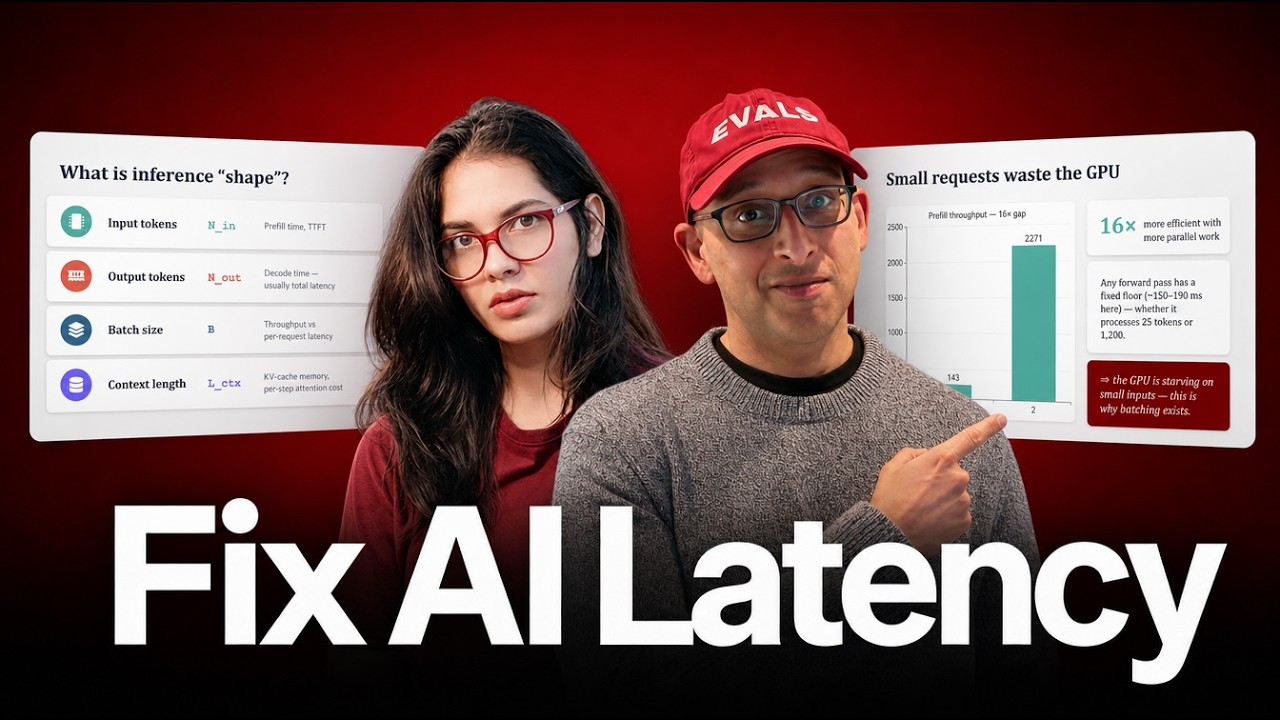
So today I want to start with one very simple problem which happened to me 2 years ago. So for the next 40 minutes, we're going to build a mental model for where inference time actually goes, and then we are going to prove it. So a little bit of update, which is I'm an influencer for a stealth startup. I'm still the founder and advisor for Apply.AI, but I'm no longer working full time on that one. I'm currently leading research in distributed systems for HPC at NOYMS, which is the school that I'm also doing a doctoral degree in, and a huge focus of mine is around fault tolerance and consistency design. So let's skip this. So here's the two numbers that I was talking about. As I was running the model, the request 1, well, it took 3.3 seconds. Request 2 took 38.8 seconds. So that's approximately 12 times. There was the same Tiny Llama model, the same T4 GPU, the same inference code. There was no batching tricks, nothing ever. And the reason I'm telling you this is I want you to sit with this question for a second, which is why does it look so different? Why does request 1 and request 2 look so different? So most people's mental model of an LLM cost is basically like if you have more tokens, that will mean more full stop. But that's not essentially true. And by the end of this talk, you'll basically understand why these requests were shaped completely differently and you'll be able to predict when would you see this gap from the shape load before you ever run anything in production. So keep this slide in the back of your head. We're going to reveal exactly which request were this in the demo itself. But to explain you why this difference was happening, we'll have to establish a little bit of vocabulary. That vocabulary is an inference shape. So what an inference shape is basically these 4 things, these 4 variables, the input variables, which is the number of tokens that you're feeding it, the number of tokens that you're generating, the batch size, which is the number of requests that you are running concurrently, and the context length, which is everything that's currently visible to attention itself. So as you're looking at these 4 numbers, it's very easy to forget these numbers when you're in the application code. And the reason I say this is most people don't really understand where time exactly goes and which one of these is the one that gets you billed the most. So that's the detail that trips people up. And a lot of people again think of them as interchangeable, but by the end of this, you'll understand they're not really interchangeable. Interchangeable. Each of them exist for a very specific reason. So that's the vocabulary we want to start with, because anytime you're looking at a real workload, it's not picking up the shapes randomly. They cluster into a couple of patterns. So what are these patterns? There are these 4 patterns with most of the LLM applications out there, which is the chat. Well, that's roughly balanced, which is you have 1:1 ratio. Input is 1, output is 1. RAG, on the other hand, is lopsided the other way, which is you're stuffing 8,000 tokens, let's to get 100 tokens of answer. So that's almost like 20:1 ratio if we're being honest here. Now the creative writing, that flips this ratio, which is you have a tiny prompt, but you're doing a long generation. And then there's the agent text system. This is the most interesting one. I want you to actually look at this one because it's not like the other 3. Doesn't ever have a fixed ratio, which is one of the reasons workloads that is hardest to predict in production. So the shape of your request really matters at this, and the shape of an agent's request at Step 6 literally contains every single thing that happens in step 1, 2, 3, 4, 5, everything up to step 6. So it's not a static shape, it's a growing one. But before Ajax, every one of these 4 shapes, no matter how their ratios look, is still built out of 2 phases. So the 2 phases that you would have heard about on social media itself, which is everyone knows this basic detail, which is what is a prefill, what is a decode. These are the 2 parts or the two phases of an inference request. So CreepL takes your entire prompt, processes it in one forward pass. Every input token will attend to every other output token all at once in parallel. Now that's the entire point of the Transformer architecture being non-recursive on the input side. Now the output of that pass will be the K, V value pairs, which is the key-value pairs that happens for every single layer for every single prompt token. Stored so that you never have to sort of recompute them at any point in time. This phase, because it happens all at once. Now when I say this happens all at once, that's not the standard, which is there's more optimization strategies that have come up, but you have to start with understanding them as different phases that happen one after the other. So now let's look at phase 2. Another thing which I wanna mention here is the reason this becomes compute-bound is this is the phase in which we are doing the MACML operations and your GPU essentially gets saturated in this phase. So another thing that you would have heard about very recently is agent systems are bottlenecked on the CPUs, not the GPUs. So that's where the agent system service comes in. So this is the phase that scales with number of inputs, the n_in variable that we were looking at. It's the phase that users experience as time to first token. So one question, you can write down in comments, have you ever wondered why did FDN streaming speed are reported as two separate numbers. They're often different. A lot of people don't know the difference between those two. So the TTFT comes from the prefill stage. Now the second stage, which is the decode stage. So after prefill, you generate one token, feed it back, generate the text, feed that back in. This is very sequential, which is there's no way around it, and that's autoregression. But here's the counterintuitive part. If you're thinking about compute-onboard modes, every single one of those jets has to stream the entire model suites plus the growing KB cache, plus the memory cost to be able to produce single token itself. So for example, if you're looking at this TinyLlama model itself, that's 2.2 gigabytes moving across the HBM bandwidth for one token. So this phase isn't compute bound, this becomes memory bandwidth bound, and it scales with the N output variable that we were looking at out of the setting variables, which is the number of outputs. This is often picked as TQUT, which is type or output token, also sometimes referred as the streaming speed. If you take exactly one fact away from this talk itself, it's this, which is pre-pull and decode are not the exact same thing. It's basically called differently. There's a very different reason for why we call them differently. Both of them have very different bottlenecks as well. There's very different optimization strategies because of the optimization that you're doing for the kind of workload that. One will be optimized on CPU, which has its own constraint. One will be optimized on GPU, which has its own constraints itself. And CPU is not just, or a GPU is just not another faster CPU. I think that's one basic fundamental here. So let's put this contrast side by side before I make any claims out here. So in the Prefill stage, you have every single thing is running parallelly. Again, it becomes compute bound. It shows up as TTFE. In Decode, it's one at a time, or the bottleneck becomes the memory bandwidth itself, and it's soften experience as the teacher. Now let's do this. Before I show you how this is going on, maybe let's look into the code itself, which is where exactly is it coming from. So we'll directly go at this stage. So this is the notebook we're going to open up and we'll start to run the cells, the first one. So before we go into the execution, these were the 4 things that we essentially talked about, and this is where the number of total tokens do come from. As we start implementing this, what we are looking at is basically the request thing itself, which is why would there was a request which was request B that was taking 3.3 seconds and what was the other request that was taking 38.8 seconds for the same model with the same infrastructure itself. So, so that's what we are going to observe. And there's a reason why we are trying to observe this, which is this is where the latency is coming from. The second thing is we want to understand how does cost work. The third thing is capacity, which is how do production systems do the prefill and the decode stages. Separately, and also the optimization part, which is all of the optimization strategy that you've most likely heard about— disaggregated prefetch, continuous batching, prefix caching, quantization. Every single one of them builds its fundamentals from exactly this. So on this first part, what we have is basically Hugging Face Transformers. The reason what we're basically trying to do here is we are trying to run Hugging Face Transformers in eager mode, plain PyTorch forward passes. There's no VLLM, there's no TGI, and there's a very specific reason for this, which is first thing is, well, I agree on this, which is ReLLM is the right tool for production. If I knew every single one of you had a GPU and the right code installed, we would most likely be doing it in ReLLM itself. But there's another reason itself as well, which is it doesn't load cleanly on a live demo on within Colab itself. And this other more important thing is it hides the prefill and decode split on an optimized server. So what I want you guys to see is first see the loop. Now, as you understand where does the prefill and decode time is separated, then it becomes very honest, which is you'll know why exactly the LLM or why SGLang or why Dynamo and all of those sort of exist. Once you've sort of implemented this, there's just one change you'll make, which is change up this first code itself, which is all the Transformers code. You would just do pip install vllm and everything would run exactly same way. So right now what we have is this very simple model that we are going to work with, which is we have a simple device, it's a T4 Tesla, and we have this much GPU available, but load up a very small tiny model, which is our Tiny Llama model, which is 1.1 billion chat models. So it takes, it has 1.1 billion parameters. So in FP16, that would mean 2.2 gigabytes in VRAM. So we can store it quite easily on the system itself. So as we have loaded this, this is the core inference functioning. This is what we are exactly looking at. So look at this part, which is the first part, is we're synchronizing everything with the clock itself, and we are writing our first inference function. As we are writing this inference function, there are two parts, which is the prefill phase and the decode phase, which is— this is the prefill phase itself, and this is the torch no_grad. This is the prefill phase that we are trying to look at, and this is the decode phase that we're trying to look at. Now, the reason we're looking at these ones is What we want to understand is, okay, so how much time does the system have on the prefill and the decode stage? This is the loop that we're exactly looking for. So we've done this part and what we would be printing is these variables, which is the number of input tokens, the number of output tokens, the number of the prefill time and the decode time and the total time itself. So what this does is it synchronizes your system with the GPU clock itself so that we know exactly how much time on the clock itself was it taking from the exact previous step. That it was running. So you would have it more like every single time what you would have is this is the number of time it got checkpointed. It took 24 seconds, it took 28 seconds. So there's wall clock time and then there's GPU clock time and less than 30 seconds for the second one. So there's a simple sanity check that we have run on this setup itself. The reason we are running this simple sanity check is what we want to see. This is more like, think of it as a smoke test. I would really highly recommend every single time doing this. So we sent out 22 tokens and we outputted basically 8 tokens itself. The prefill time was 152 milliseconds, ms, which was 144 tokens per second. The decode time was 7 tokens per second. Now notice one thing, which is how the decode time is much lower than the prefill time. It's for the same model, for the same GPU, different phrase, different bottleneck. So the reason we are trying to do this is we are trying to warm up the GPU so your experiments won't pay the start text every single time. This is one of the big problems in production, which is companies try to push the models in production before investing in a stage that does the warmup. And what happens initially outside of that is, okay, it takes far too much time to load and destroys the SLAs. So that's the part that we are trying to avoid with this. Now on the second step, we are basically doing 3 small experiments. So our experiment A, we're using a very tiny prompt, which is a simple prompt, explain what a GPU is in one sentence. This is about 25 to 30 tokens. And what we are saying is basically give us a small output of this one. Now on the second one, we are giving a long prompt. The reason why we are doing this is we are trying to see all of the shapes that we were looking at earlier, which is on different shapes, what does the ratio of the input to output looks like and how much time does each of them take. So I can run this again, but you can try running this as well. This is— I just executed it before the call itself. We have the creative prompt itself. Right now we're not looking at the Ajitex system, we're at just the RAG, the small one and the big one in the creative one. And we're looking at the number of input-output tokens. As we run these experiments, we define what we are basically going to call them. So let's run these very simple experiments as we do this. So for the first request that we were looking at, which is the small input, the small output one, our parser time is very relatively short, which is it was just one line that we basically gave to the system. So it gave us 40.5 milliseconds. The decode time was much bigger because we we asked it to sort of explain it. Again, it's not massive, but it's reasonable. So as you can see, the main difference, which is the decode, is the one that was taking majority of the time here at this point. And the prefill share on the GPU itself, or on the total latency itself, is 4.3%. Now on the long one, this is the number that we want to look at, which is the prefill time is bigger because again, we gave the long context itself on the RAG itself. The decode time was much reasonable, I think, especially for this one. So on, on this, we gave out a long prompt and we said, and the third shape that we gave out was basically when we had a short input and a long output. So when we gave a short input, the long output, as we can see, the prefill time was very, very small and the decode time was the major one. So the prefill share was actually very little. Now this is the first part you guys are looking at. As we try to represent this, these are the shapes that you are really looking for, which is how much time does prefill and decode. In the short to long And blue is basically literally invisible. In this one, it's close to invisible as well. It only is visible very much in where we have the RAG system. So this is what you're looking at. The second thing is the latency share by experiment itself. Now I don't need you to memorize these patterns, but the reason we're looking at these patterns is so you can very quickly start seeing if I'm going to give a very long or very short prompt, how much latency is each stage going to take? And once you know, okay, this is the latency that I'm working with, then you can start working on how do I start optimizing for those stages essentially, which is, let's say your prefill is Compute Bomb, then you would start looking at my prefill is taking, let's say, 432 seconds in the latency period itself, which is, that's the latency it's taking on my system. Now you would start looking at, as you start doing prefill optimizations, you would start using that number as your baseline. As you're looking at decode, you would start using the decode number your case, like that's the reason we are bringing this system itself. So this is the first plot. Yeah, look at these numbers and then you would very quickly see which is what was the total time taken was 7,000. Okay, interesting. This is the long in short out. So this is one thing where people make this confusion. Okay, so this is the one where we had the short input and the long output. That is usually the one that has the longest latency and not really a RAG system. Why so? Because the latency was generated now by the decode taking up most of the time doing these sequential computations itself, because the prefill was not really doing sequential computations. This was the part doing sequential computation. So when you make this part really massive, then again, that starts impacting. So every single time, think about it this way, which is most of your latency will 99% of the times come out of whichever one has highest decode stage itself. Now let's look at the numbers itself, which is So what were we measuring? So this is the case that we were just seeing right now, frozen in chart. There's one line I want you to take from it, which is the prefault share of total latency was 3%, 16%, 0.5%. At this point, the decode wasn't really a factor latency. So one, again, I think I've already said it, but decode will be your latency. So now let's look at one actual number, one of the other things where the latency comes from or why this asymmetry sort of happens in your system. Well, there's there's a small token gap here. In our experiment B, what we were looking at was 1,205 input tokens that were prefilled at 530 milliseconds. That's about 0.44 ms per token. Now output tokens were roughly the same. Now do that division once very quickly, which is it's 300 times more expensive in wall clock time to write a token than to read one. So the writing is where most of your time is consumed on the GPU clock as compared to, or even in your entire system itself, unless you're using a really bad load balancer as compared to the time reading a token itself. The pricing page that you want to look at, which is anytime you're looking at pricing, they would have these two numbers written very separately, which is this is the cost for your input tokens, this is the cost for your output tokens. So anytime you're making that pricing decisions, think about it from that perspective itself. Now anytime we have small requests, it ends up wasting the GPU, which is— this was another thing that ended up falling out of the same data itself, which is the request number expiring C, which is we had the prefill throughput, which is the tokens per second. Now in our experiment 1, we took 143 tokens per second. Our experiment D, we took 2,271 tokens per second. That's a 16 times difference basically in the same phase. Now what I want you to do is to flip that around. With only 25 tokens, you were leaving the GPU almost completely idle. So what happened was your GPU was actually stopping. And that observation is why inference engines do exist. This is literally what most of the inference engines, VLLM, Mistral Lang, or any of the other ones try to do out there, which is this part of the process is called continuous batching. So throughput happens to be one resource that you can waste. And what VLLM tries to do is it tries to batch as many pre-filled tokens as possible within one single request. So you end up not wasting too many requests or too many processes is giving out very small tiny requests. So the execution, if you look inside the code for VLLM itself or within scilang, there's a file called scheduler.py. So that is exactly what's doing this part, which is stopping the small request from wasting a GPU that's capable of now handling 2,271 tokens per second. And this is the part that would have been hidden if we would have tried to use VLLM, right? Now let's talk about one more number here. So the other number is the KVCache. What KVCache does is is we didn't look at KVCache in this very particular example itself. KVCache was generated from the AgentX system, but what it really does is it's the memory that's growing per output token. So what a normal system basically says is, well, you're storing your keys and values for every single attention head, every single layer that we're plugging in the TinyLlama model itself. TinyLlama 1.1 billion model, I think that we're using. So for each of those ones, you get about 0.17 megabytes per token, sort of measure the KVCache. But there's a very simple formula for it. Now what happens is this number, as we do this measurement towards the ending of the code itself, as we run the code lab, this number turns out to be much smaller than the theory predicted. So I'll show you why this is interesting. Maybe this is the second thing which I want to show you. A lot of people say, okay, Kiwi Cache is eating up all of the memory in our system, and that is one thing that you need to plan out for. Again, why isn't it as scary as most of the people think? But before that, let's go into AgentX system itself, which is— let's go into the AgentX code. So what we've done is we've simulated a multi-step agentic loop. Again, this is a very simple implementation. What you can do here is you can use QAI or anything else, but in each step, what we would have is we would be generating a prompt, we would be running an inference, and we would be appending the model and the history that came from the previous prompt to the model itself. The problem with frameworks is they try to introduce a lot of latency in your system, and I want want people to sort of very quickly see where exactly is, how many tokens is exactly every single thing consuming itself and not get bogged down by the complexity of we have to use this framework or we have to use that framework. Another thing you would very quickly realize once you start building out agent systems is most of the frameworks are fantastic for you just getting started, but once you're building production systems, they start failing very quickly.

I totally agree. Yeah, like even updating the prompt in some of these frameworks really weird. It's like 3 abstraction layers down, there's some hidden prompt somewhere. It's just like very complex.

So one of the things is at every single point in time, what we're doing is this step, we are resending and refilling the entire prompt history from scratch. So the agent isn't remembering anything. We've not built out the context graph or we've not built out the memory part. This is much simpler implementation of this one. So what this means is is it will reread its own transcript every single time it wants to take an action. What that really means is think about it in terms of runtime, which is every single time you add up more input tokens, your runtime will start increasing in a sub-quadratic manner, which is O, again, the fun input itself. So on this one, what we would be looking at is the very same things that we tried to look at earlier itself, which is the number of input tokens, the number of output tokens, the total tokens that were taken, what was the time in the prefill, the decode stage, and what was the wall time that was taken. So this is what was generated by a very simple AgentTech script itself. So what we have is this system essentially took 5 steps. The number of input tokens were this much, but what we are interested in here is the prefill time and the decode time. So as you can see very quickly, which is the prefill never ends up taking most of the time. In an Agent Mix system. It's mainly the decode time. The reason for this is decode is adding up after every single step out there. So the total wall time is this. So the prefill ends up taking only 3% of the Agent Mix system's latency. And this is very clear when we talk about the prefill stage itself. That's the prefill that is being generated by this particular system. If you have a lot of tool calling that is happening, again, the latency can sort of increase. So let's try to visualize this very quickly because Ajitik systems are not just an input-output. They have 3 more variables that become very important very quickly. One is the batch size. The other is the context window itself. And the third thing is the number of tool calls. So if you're looking at these graphs, essentially what you would see is the context growth was happening across the steps itself. And first step prefill versus decode latency, if you're seeing very quickly, which is the prefill. Still straight nominal at every single step of the way, but it was the decode that was increasing. Now, how this graph changes, which is why is the center one bigger than the last one? Well, that's totally random. That's just because of the kind of script that we have written. This shape can essentially end up changing every single time. So your overall latency coming from the pre-filled system was very little as compared to coming from your decode system, and your cumulative latency, which is the green line, the green line is the one which just closes the decode. So again, I think one more system to sort of explain that your latency will may come from the decode stage. Now how do you start calculating up the cost itself? Which is what you do is now if you have a GPU system, well those costs become quite obvious. But if you're looking for an API itself, well for this one I've used the OpenAI numbers. So the input token, the output token, and what I've done is calculated up the cost from this perspective itself. So a single chat request, which is a single flow, only ended up taking this much dollars, but a 5-step agentic loop ended up taking 11.9x more. So this is the part where you could sort of assume, which is the number of steps, as you increase the number of steps, the cost will increase. But where is that cost coming from? Again, the decode stage, not essentially the prefill stage itself. And this is the fun part, which a lot of people get wrong. This is a very simple way of looking at how the memory growth was happening across the KVCache itself. So across the KVCache, what I've done is I've started looking at what were the input tokens, what were the output of it, how much prefill was being generated. And for every single prefill being generated at every single step, I'm storing that as the prefix value, as the KV cache itself. So if you look at these numbers, this is a very counterintuitive graph if you look at it, which is this is the KV cache memory that was actually being used. And a lot of people assume this must be the number, which is this is the number that would have been our KV cache growth. KV cache growth doesn't really happen this way. There's one very particular reason for this. Is if you come back to this slide, here's the same graph that you're looking at. The reason for this is different models do have different architectures. So for example, Tiny Llama model that we're using in this very particular case uses a strawberry attention, which is the number of heads and how each head will generate PV cache itself. There are models, for example, MOE models, and there's MLA models. Every single one of those particular categories of models, and that's where you start looking at what is the essential architecture. Is it MQA? Is it MLA or is it MOE architecture? So in this one, TinyLlama model is a GQA model, is a Group Query Attention, which is for a group of KV value pairs. Those KV caches being generated as one and that's stored at basically one head. So at every— there are a couple of requests, there are a couple of KV values that would be storing or sharing this KV cache itself. So what happens as you group of this is you end up taking less memory within your system as compared to what would have taken— the memory that would have taken if every single head was generating its own KV cache itself. So think about this as the context piling up anytime you're using or anytime you're looking at a model out there. Now another thing I want to mention very quickly here is as you're looking for which model to start picking up, ideally you want to pick a model that is grouping up the queries, that is grouping up the intention that is grouping up the KV cache itself. So MOE models, for example, there's another one, I think the DeepSeq, they have a 24 billion model. I think they have a 15 billion model as well. One of the biggest reasons for the MOE models to be able to generate less KV cache is basically this thing, which is they group it at this depth. And that's the reason you're seeing this kind of graph out there. So now coming back to the agent cost itself, so if you're seeing this, a single agent versus the 5-step agent that we ended up building this. So we had 11.99 times the cost. This was not the latency, this was just the cost itself. So look at where this value is coming from. So most of this value was coming from the tokens that we were generating as comp— in the subsequent steps as compared to for like a single turn. Any inflation that you're seeing in your agent text system that's the resync input. So every single time you're resending your input back into the system, that is where the cost is coming from. So the lower number of tokens that you can send in your input back to generate the decode, that is essentially what decreases the cost for a model itself. And that's what you're trying to optimize for when you're trying to build an inference system, which is what's the smallest amount of KV cache that we can share back with the system to be able to do the decode generation. So if you're running agents at any scale, this number, the number that we are looking at is where most of the cost will come from. And this is not small number, which is even in just 5 steps, this is 12 times. So this is the big difference between what becomes more like a line number within the balance sheet itself and what makes your feature end up getting killed in a budget review. So we've covered 5 very dense ideas. Let's look at all of the ideas that we talked about today. The first thing is the latency lives in your decode. Now output tokens are almost always roughly 2 size orders of magnitude more expensive than your input tokens. So that's how you want to do your calculation at any point in time. The second thing is TTFT, which is tied-to-first-token, is a prefill story, but total latency is mostly always an output line story. So you want to control latency, cap the number of maximum tokens. Don't just tune your retrieval pipeline. That's going to do very little in what you will be able to achieve. The third thing is if you're making very small requests and sending them to the GPU, that will start the GPU. So what you're going to implement here is batching. So instead of using 143 tokens per second, instead of giving that to the system, instead give 2,271 tokens. And this is where you can write your own batch function. This is where you can do optimization on top of VLLM, on top of SRELAB. Every single one of those inference engines out there, although they are pretty much optimized. But again, that's, that's one of the areas of work that you can essentially work on. The fifth thing is agents read by their entire history every single step of the way. So the context management part, that's not just optimization for agent products. That's what will make the difference between whether you're building a system that would survive or whether you're building a system that will eventually get yield. Now that's the entire thing. I think I'm going to give you a very tiny homework. Um, I know this is supposed to be a lightning talk, I'm not supposed to give you homework, but I want you to do this, which is right now it was using a single batch size, which is batch size 1. I want you to start playing with batch size 4 and batch size 8 and see how much difference does the prefill and decode latency generate. The second thing you're going to do is right now we were using Hugging interface. So if you're working on a Mac system, there is a small possibility you will have troubles installing VLLM, at least the 12.13 versions of VLLM itself. So start with maybe llama.cpp itself, install it, and then see how much prefill and decode latency is being generated, because that does batching automatically for you, that does the scheduling automatically for you. Then start swapping different inference engines and how each inference engine affects the prefill and the decode stage. Now the other thing we did was for this particular model itself, we used an FP16 model itself, which is the Tiny Llama model that we were using was an FP16. Try to use a smaller quantized model here, which is using int8 or int4 of the same model itself and see how much the prefill and decode are taking up space on the memory itself, how much latency each one of them is generated and how much cost would you be generating at every single point in time. And the final thing is the prefill prefix caching itself. You don't have to do it yourself from scratch, but look at how— what is the smallest amount of KV cache that you can give to the system. Maybe you can design a fantastic system around it. If you can't, then use VLLM, use SGLag, and look into how they are doing this basic part. So this part is done within— there are two files that they are executing this in. One is called a batching or a batch.py file within the LLM. And the other thing is the paged attention. So that's where the prefix caching is happening in the system. And that's where, why the paged attention, flash attention algorithms have become so helpful. And that's the reason everybody's talking about it. And one of the things I'll say before I wrap this up is those are not the most optimal algorithms. Those are not the most ideal ones. They're sort of optimized for most of the models out there. There, but there's always a trade-off, which is I think what they're trying to reach is this works on most of the systems out of the box as compared to writing a kernel for every single one. So think of Flash Attention as a kernel, which is very specifically written for optimizing up the 5 parameters that have exist on a GPU that we are looking at, which is on the silicon itself. For every single model, you can start optimizing up those kernels and how quickly they do the MACML operations. And that's where kernel engineering Okay, so now you know the shape of the request, where your Python money is coming from.

You work on inference a lot with a lot of different companies, and what are the common mistakes that people are making even despite using VLLM, whatever, out of the box that kind of come with best practices? What are the mistakes that you see most often, especially like low-hanging fruits nowadays?

So the first low-hanging fruit, like I said, the sanity check that we try to do today, which is most companies, what they do is, okay, we've built the most fantastic model, we have trained it, let's put it in production. So they don't spend time testing out or warming up the pods and warming up the setup itself or the infra itself. That's where a lot of systems do get shocked, which is that part in itself requires checks and balances before you hit ready, before your GPU basically says hit ready on the system. So that's the first part. The second thing where I'm seeing a lot problems happen is the way models are being distributed on different pods itself. So what's essentially happening is companies are trying to carry the same model on different pods and what they're not doing effectively is the KVCache sharing between these different pods itself. The third mistake I'm seeing happening, and this is not a mistake but more like an open problem, which is how much KVCache are we going to store? How long are we going to keep it? Keep storing up the KV cache in the system before we start removing it? Because that sort of deadweight, like after a period of time. And that's a similar question which DuckDuckGo, which all of the database companies were asking, which is how long do we hold the memory within the system for our system to be able to work optimally? As companies are trying to own these systems themselves, which is as they have these GPU systems on their own premises, most of them I don't see clearing out the KV cache. At any point in time, which is they're just holding and holding and filling up the GPUs with just KB cached itself, which after a point becomes sort of useless, very similar to how the drift happens, which is now the most relevant things sort of become more important.

That's really helpful. Okay, the next question is, a lot of people are interested in open models, specifically from like ownership perspective, privacy, and then cost, but how should people go about about thinking modeling the cost, meaning like how do they know, do they have it like have enough volume to like justify hosting their own models? Is there a way that you kind of like to think about it?

So there's two perspectives here. One is the cost perspective, one is the regulation perspective. Because I live in Europe, so the regulations are the one deciding factor where companies are saying, okay, no, let's just host up our own GPUs. Where I'm seeing in the US, where specifically with the companies I have worked with, is there's a hybrid approach that's working, which is for most of the training that happening on the systems, or, and even for, so if you're making the small request, which is the one-time request, those are being handled majorly on, uh, using their APIs, using other people's GPUs or using inference GPUs from ModelLM and all of those companies. What they're trying to build is for the long-running agentic system where you have multi-step calls. Ideally, they are trying to run it on their own GPU, so they're not adding up the cost without having some sort of supervision around that.

Okay. The next question I have is, so We learned today that decoding is going to be the thing that takes a lot of time no matter what you do. And I think a lot of people have heard of speculative decoding to maybe help with that. Do you have any thoughts on that? Is that, is that good? Is it easy to implement? Is there any footguns there? Second question I have is like diffusion, diffusion models or any other kind of techniques, like is it worth exploring those? If you would talk a little bit about that.

Okay, so I think the second answer is very easy, which is I don't work on diffusion models, so I don't really know what happens in that territory, I would love to know. I'm just working on LLM sensors, going towards— I've done some optimization for voice models as well, but I'm going towards the multimodal stage where I not yet build the competency in vision models. The first question, which is what about speculative decoding? So where you see techniques like speculative decoding or disaggregated people, all of those techniques are built up majorly for this reason, which is for 1.1 billion model, the prefill and the decode stage are not massive. But if you have a way more massive model, think about it as like 45 billion is your initial beginning limit. At that point, your decode requires a lot of KB cache itself, which is for— because you're generating KB value pairs from every single stage itself. So speculative decoding and all of those techniques were basically created to keep your KB cache controlled. Where you would think about those techniques is anytime you have more than 45 billion models, start thinking about how can I use a disaggregated prefetch. What disaggregated prefetch basically means is instead of the prefetch being one long drawn stage and then the decode starting, you break it down into small phases, which is one prefetch, couple of prefetches. Now it starts generating decode, then it keeps generating the prefetch, it keeps generating the decode as well. So it becomes more continuous and it happens in batches. Same is true for speculative execution. Of decoding, which is it's a process where you're trying to optimize for the decode stage itself, but it's not a major concern for smaller models. It's not a major concern when you don't have the big KB cache increasing. So it's majorly to handle that problem itself.

Before I turn over to the students, I think it's worth asking, okay, so I think you've piqued everybody's interest in inference optimization and like all these different components. If someone wants to learn more about this? And because you do so much work on this, like, where should they go to learn more?

If you don't have any background on building ops solutions, then come to the Forward Deployed course because it starts from like a more simplistic place for people who are data scientists who come from that kind of background. If you've already been building ops solution, if you already have the decision power within your companies to say, okay, now we're building up the platform side, if you're really in those platform roles where your focus is not really on building the agent systems. That's somebody else's job. And you're basically told, now we want to serve this to 1,000 or 50,000 clients every single day. That's where you come to the other course, which I have on inference engineering systems design. But again, you don't have to. Just, just putting it out there. I think I'll give two more resources as well, which is if you don't have any background in the space and if you're interested in learning the fundamentals, interested, there's a book on inference engineering by Philip from Bayes Den. That's a fantastic intro book, I would say. You can pick up that book. The other book, which is on AI systems performance engineering, I think it's called Systems Performance Engineering or AI Systems Performance Engineering, it's by Chris Freckley. That is the book if you're focusing very much on going towards kernel engineering side. So there's the middle part, which is— I'm sort of writing for, but you have those two spaces that are already covered up. So you're trying to build up systems for NVIDIA, there's a very good chance that you would be working very heavily on Blackwell architectures and how can I optimize the infrastructures with very specific algorithms itself. So I think Chris Gregory's book would be one you would go at. The other resource I have is there's something called gpengineering.com. So there's a website. My own favorite book that I started learning from, from almost 3.5, 4 years ago is the PMEP book, which is one of the classics in the compiler Dragon Book. So a lot of my coming from there. I have notes from those books as well on the website itself. So go on jpenjerdane.com, you'll find the book, the notes, and notes there.

All right, thanks everybody, and thank you so much, Abby, for coming.

Thank you. Bye-bye. Have a good one. Enjoy.