#6 Supervised Machine Learning Full Course: NumPy Code From Scratch
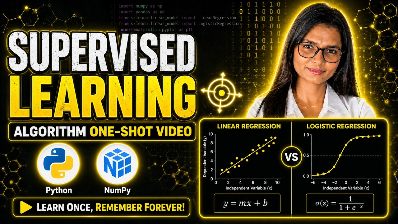
Akansha Yadav builds linear and logistic regression models from scratch using only NumPy, covering the forward pass, loss computation with Mean Squared Error and Binary Cross-Entropy, gradient descent, and hyperparameter tuning. She clarifies that linear regression handles multiple features and non-linear relationships, and that logistic regression is classification despite its name.
Chapters
So hello everyone, welcome back to another exciting video on supervised learning. Yes, this is another part of machine learning series. In this video we are going to discuss about supervised learning algorithm. What is it? What happens behind the scene? Which model to choose? What are the different type of supervised learning model? And many more things we are going to cover in this video. So if you have anything in your mind, this video is going to clear each and everything. If still there is something which is left, then do let me know in the comments. I will surely handle them. Now let us begin with supervised learning algorithm. You might have seen so at so many places that, okay, these days we are using applications a lot. We are using Instagram, we are using YouTube, we are using a grocery application and even food delivery applications, right? Let's talk about Zomato. How does Zomato know that when your food will arrive? Yes, Zomato generally used to show us that, okay, in 32 minutes you are going to get the delivery. 'in 44 minutes you are going to get the delivery.' How does they get to know that? What is the exact number? How can they display this number? And this also happens that, okay, first, at first it was showing 32, but then it showed 35. So it means it can keep on changing as well. So what happens behind the scenes? So basically, Zomato uses supervised learning algorithm. Yes, Zomato uses supervised learning algorithm and has trained its model on the previous data. So it works on 3 things, right? So first thing that it works on is how much time is required to cook the recipe or the food ordered by the client or the customer. So it means kitchen timing it takes, right? Cooking time, how much time will it take? Second is the traffic, that the location that we are trying to deliver the food is at what distance, what is in kilometers. According to the kilometers, it calculates, then it checks for the traffic, right? So that's the second parameter that it works on. Third is the packaging time, that how much time will it take for XYZ per person to package it, right? To make it look good and deliverable, right? But there is still an accuracy and limit with the models, obviously. So maybe sometimes the traffic is high, or maybe the road is not that smooth to deliver the food on time. So they keep on changing the value of minutes, they keep on delaying, right? So this happens, right? But every machine learning model has this accuracy and limits. So this is not something new. Zomato is also going through the same thing, right? So accuracy and limits remains constant with every machine learning model, but what we get as a gift is the predicted value, estimated value, right? And that estimated value is generated with the help of supervised learning model, right? So Zomato is using supervised learning model to give you the predicted number of minutes, correct? Now, we have already discussed about supervised learning in the first video of our series, that what we actually do within supervised learning is we use the same human brain method for models. It means just like how we were getting trained, we were doing the same thing. It means if I get to know about apple is via my teacher, right? My teacher have shown me multiple pictures and have told me, okay, this is apple, this is banana, this is grapes, right? So it means I get the picture also and get the label also, right? Same thing we do in the supervised learning. We give apple, banana, grapes data to the model. Model fa— model basically eats that thing and then gives you the predicted output, right? This is what happens in supervised learning model where we purely work on data, but along with the data we also work on labels. Yes, we give labels so that our model can easily get trained, right? It is easy to learn when there is a mentor, right? It is easy to understand when there— when we all have mentors, right? Same thing we do with the machine learning model, and we use supervised learning model for that purpose, right? But throughout this journey of machine learning model creation, there are so many different tech terms which we are going to use. The number one is features. What is feature? Feature is nothing but the input. Feature is nothing but the input variable, the information that we have, like what is the person's age, what is the salary, and the experience. Based on age, salary, and experience, I want to predict whether that person bought the car or not. I want to predict that if that person is of 42 years old and have the salary of 85,000 with an experience of 10 years, will that buy a car or not? Yes, obviously, right? So based on the data, based on the features, based on the input variables, what do we do? We predict some things, right? So first term is the features. Features are nothing but the input variables for the model. The next is labels. What is label? Label is nothing but output. What are you exactly trying to predict? Okay, the thing that you are trying to predict is label. Label is the target variable that you are trying to predict, and you— it can be anything. It can be number, it can be category, Anything it could be, but you should know what is your label, what is the final output that you are trying to predict. Next is observation. Observations means how many number of rows do you have, 15,000 or 15 million. So that is observation. So these are the 3 terms. Now let us understand features. What are the different type of features that you might get? So features can be area, bedroom, location, blood pressure, sugar.. So based on these terms, these variables, what all can you predict? It is just nothing but the information that we already know about that person, right? So these all are features. So whenever you are confused, just ask yourself, what information do I already know, right? Next is the label. Label is what are you trying to predict? Based on the area, bedroom, and location, I can tell the price of the property. That, okay, the area is, let's say, 1 acres, number of bedrooms, let's say, 10, location, let's say, XYZ. So I can tell the price. It means what I am doing is I am using the input feature to give the output, to predict the label, to predict the label. Same way, age, sugar, and blood pressure can help me predict the person is having a disease or is healthy, right? Same way, in school, we see how many hours you are studying, then test scores and the attendance tells us about pass and fail, right? So what are you trying to predict is your label, right? Next is the target label. Your target label is something that tells the next path. It means whatever you are trying to predict will tell you which model to use. Yes, that's correct. If you want to predict a continuous value, if you want to categorize something, if you want to predict someone's next move, what is the number of minutes that the food will be delivered in. So whatever is your target variable or target label even you can call it, that tells your path forward. So in supervised learning we use two types of models. Which two types of models? We use classification model and regression model. Yes. We have only two type of supervised learning models, right? One is the regression, another one is classification. As the name says, classification means classifying something. If you want to classify anything in like, let's say, spam, not spam, so this is also one example of classification. In regression, we have a numerical value. When you want to predict the temperature, that what will be the temperature after one hour, what will be my body's temperature after one hour, right? So it can be anything.. So when there is a term called numerical value, when you are dealing with numerical value, you go via regression. When you are dealing with categorizing, go with the classification, where— which will help you to classify, right? Let us move ahead. Regression, as I told you, regression means working with numbers, working with numbers. So when you are working with numbers, and there can be infinite possibilities of the output— numbers can be infinite, right? Numbers are infinite, right? So regression is something when you are working with a numerical value, the numerical value which is continuous. It cannot be a fixed, right? It has to be continuous. It means we are going to deal with fraction and decimals. We are going to deal with fractions and decimals, and there is no fixed limit. Now in regression, if I— if you ask me the examples, then temperature is one of the example as I have given you, right? Delivery time, which we are, you know, discussing since the beginning of this video.— that how much time will it take, right? Then rainfall amount, is it going to be heavy rainfall? What will be the percentage and so on? Then salary, employee salary, house prices, and everything is basically related to the continuous numerical value. Therefore, we use regression model for this purpose. Then for remembering what exactly regression means, numbers. Regression means number. Just remember, number means regression, and that's it. Next is classification. As I told you, classification means categorizing. Where we work with 3 things, where we work with 3 things. Classification is used when you want to categorize it in category, class, and labels. When the outputs are not basically the fraction, decimals, or numbers, or a continuous number, they are only the 2 categories, 3 category, 4, or many more categories, but just the category or classes or labels. Then we use classification model. Now there are many examples like spam, not spam, fraud or genuine, or there can be images which you wanted to classify. So every time if your output belongs to category, it means that is a part of classification model. This is also important. Next is there are further types of classification models. Yes, regression is regression. Continuous number means regression, but when it comes to classification What do you want to classify? Is your output binary? Binary means 2, 0 or 1, right? Same thing we do, exactly 2 possible classes. It means spam or not spam, fraud or genuine, are the part of binary classification. So for binary classification, we have a different set of algorithm. Then next is multiclass. In multiclass, we have many possible classes, but output will be 1 only. It means If we have an image and there are multiple containers, you have to categorize it in. This is for dog, this is for cat, this is for horse, and this image is of horse. So obviously this image will fall into this category, not going to fall in all of them, right? So this output is only one. So this is called multiple class. Why it is called multiple classes? Because we are not dealing with binary. Binary means two. Now here we have three, more than two. So multiclass is for more than 2, right? Next is multilabel. What is multilabel? You remember, like if I talk about any movie, right? So that movie can have multiple genre, right? For example, if I say this movie is having comedy also, action also, and some percentage of romance also, it means that movie is going to have multiple labels. It means if you ask this X movie, is action, comedy, and let's say romance. So A, C, R— 3 different categories. It means in the case, case of multiple or multi-labels, we are going to have multiple outputs, multiple containers that output will fall in. Output is not going to be one, output is going to be multiple, right? So this is multi-label. So there are 3 type of classification algorithm. Depending upon what you are trying to classify, you will choose one for yourself and proceed ahead. So this is a set of regression models which you have. There are many more, the list is so huge, but for now I have just displayed 5 of them, right? Now one is linear regression, ridge regression, which is L2 regularization, lasso, elastic net, and polynomial. As with the name, we can also get to know that these two are based on regularization technique.. This is elastic net. This— in this we use polynomial equation. In this we use linear equation, right? It is simple to understand what goes behind the scene within the model, right? As I told you, the list is huge, but still I am just displaying only 5 of them. Next is the classification model. In classification model, we have a logistic regression, Naive Bayes, linear discriminant analysis, LDA, KNN and then SVM, and many more obviously are there in this series as well. But what I am trying to tell you is this— these set of models will help you choose one for yourself. If you ask me, this Zomato one, this uses gradient descent, XGBoost, Naive Bayes type of model to tell you how many minutes will it take to deliver your food, right? So Zomato is the best example to understand. But there are so many misconceptions which are related to the models, right, which are related to supervised learning model. Therefore, I have tried to capture few of them, and if still there is something in your mind while learning, right, this generally happens with the self-learners who tries to figure out via tutorial or, you know, watching the videos and all. So the very first misconception is logistic regression is a regression algorithm. But this is completely wrong. The word logistic regression— regression means continuous, so regression means regression category, it will go in. But this is not true. The correct thing is this: logistic regression is fundamentally classification algorithm. Yes, it helps you classify. Generally, we use logistic regression in binary cases, in binary cases. Now let me tell you why it is called regression. Why have the developers named it regression? The very first reason is under the hood it uses linear combination. Linear combination means it uses linear dot product between x and the weight. What is the weight? As I told you, what is the weightage of x? It means if I am saying 2, what is the weightage of 2? Is 2 more important than 4? Or like basically what is the weightage of the input features or the information that you are providing? Is this, uh, like solid, like is this having a large weightage or what, right? So x will have some weightage and this two has to be multiplied. It means dot product has to be, and then comes the bias. This is a general mathematical equation which goes under the linear regression type of model. So we use linear combination, therefore linear is something that comes in, right? Now next is we use sigmoid transformation. So when we talk about the final output, let's say z, Instead of directly giving the z, we try to squeeze them into the range of 0.1 to 1.0. It means real value will be, you know, squeezed into the probability range of 0 and 1. And for this, we also use class probability thresholding to make the perfect decision so that we go via classes and probabilities. So we use some conditioning to apply the class probability and threshold and try to categorize 2 stuff, right? Why it is called regression is because we use linear regression in this, and we also use logits to, you know, get the positive classes rather than working with the raw values and so on. So what I am trying to convey is logistic regression is not a regression model. Logistic regression is a classification algorithm. Yes, you can use it for binary classification. How do we do it? We will learn about it, but for now this misconception has to be removed that this is a regression. Second is, let's say you have to work with this ratings, okay? There's a product which I ordered from Amazon. Now Amazon wants me to give rating, so the rating have 5 categories: 3, 4, 5. Either I can give 3 or 5, I cannot say 3.5, right? Because I have given the 4 or 5 independent values, right?. So this is what we call as— so we call it as the values which are basically the ordinal values, like ordinal variables, right? So when we talk about ratings or ordinal values, variables do not go for regression. You might be thinking it is numbers, so let's go for regression model, but that's not true. Numbers, but these numbers are fixed. Right? So therefore you cannot go for regression model. What is happening with this board today? I don't know. Yeah, regression means continuous value. Regression generally works with decimal values, not the fixed limit. 1, 2, 3, 4 is a fixed limit. 5 independent values— when it comes to 5 independent value classification works well. So this time with the ordinal variable, go with the classification. I hope you understood. Next is the misconception which is related to multiclass and multilabel. Although I have already told you what is multiclass and what is multilabel. Multilabel means outputs are going to be many. You will categorize or you will give it multiple labels, but when it comes to classes, it is going to just have one. Label means many labels, right? As I have given you the example, this movie is action movie, comedy movie, or romance movie. When it comes to image, it can be either be dog, cat, or horse, right? That example you remember. So it's the same thing. So multi-class means single choice, multi-label means multiple choice, right? So these misconceptions we have already covered. There can be many as well, so do let me know in the comments. I will surely resolve your doubts. So first is regression means drawing a straight line. No, it doesn't mean drawing a straight line. It means when you are trying to predict the numerical value, it means predicting the numerical value. And multiclass, multilabel, numerical value, this we have already covered. So this is how you can, you know, understand it well. Classification means working with categories, getting the discrete data, and working on spam detection, disease detection, sentiment analysis, and so on. Regression means output is going to be number, values can be continuous, and you are going to display sales, salary, house prices. Now, how one can identify which machine learning model to use, right? This is something which many of you might be confused for, right? So first ask the question to yourself, what exactly am I trying to predict? Is this a continuous number or a discrete category, right? Continuous number or discrete category. Now if it is a continuous number, regression, stop. If it is a discrete category, then ask further question. How many correct answers per observation? Out of 2, binary. Many, multiclass. Many and multiple correct, it means multi-label. That's how you can identify one algorithm for your problem statement that your client or stakeholder might be asking you to do. You should be aware of what is behind the scene of the model. So we are going to create two models. We will create one classification model and one regression model using just NumPy. Yes, just to teach you guys what happens behind the scene, right? Now these are the set of problem statements or the problem algorithm basically which you can use to Choose one for your next problem statement— linear regression, decision regression, random forest, SVR, XGBoost. And then classification, we have logistic, random, decision tree, KNN, SVM, Naive Bayes, and many more algorithms are there in these series. But you have to understand what happens behind the scene, and for that reason we are going to build one for classification and one for regression. And later on we will create end-to-end projects, multiple projects for the supervised learning, and then we will switch on to the unsupervised and so on in this So now let us understand how to create linear regression model, how to create logistic regression model. But before that, let me give you the brief idea about any algorithm. Yes, how does any algorithm works? What are the training phases? What are the parts of training phases that a model goes through? So it goes through two paths. One is FP, another one is BP. What is FP? FP is forward pass. What is forward pass? We will discuss. But what is BP? It is backward pass. Now what is forward pass? So within forward pass, this is applicable to any algorithm that you are going to create. Now any algorithm, it means what it includes it, it takes the value X, it is nothing but input features. Right, and gives it to the model. Then model gives you y-hat. What is this model? This model, it can basically have different mathematical function, its steps, its own property, its own, uh, you know, capabilities and everything, right? So we give input to the model and model gives us y-hat. What is y-hat? Y-hat is the predicted output. What is a predicted output? Predicted output, it means what is the model's prediction with respect to that particular observation. So observation is the single row, right? So depending upon the single row, single input feature, it is going to predict it. Now this is what happens in the forward phase. So whenever any model starts its training, it takes the random initial values. Yes. At the beginning, in any model, it takes the random values, and those random values will be updated in the backward pass. Now, what is backward pass? Now we know that from the forward pass we have y-hat. Y-hat is prediction, and we know that y is a final actual output. Okay, so what do we do in the backward pass is we try to compare y-hat with y. Yes, we try to compare them. We try to subtract depending upon if it is a continuous value, we subtract it. If it is not a continuous value, we do not subtract it, but we compare it whether it is same or different. If it is different, it means model has probably obviously basically made an error, right? Now in forward backward pass, we take y-hat, we compare them, and we try to check if in this observation that model has made an error or not. If there is any error, then what do we do is we jump on to metrics. Yes, what is metrics? We use metrics to calculate error first. Then there are certain steps that we need to follow to get the model with the correct values. How does it happen is after comparing, we ask our model to update W and B. To update this, we use gradient What is gradient? You can watch the video which is on i icon. I have added each and every details. I have literally explained how to create one model, what is backpropagation, how does the gradient descent works, and everything which you need to understand with respect to any model, right? So we apply gradient descent. Gradient descent is applying derivative, applying some mathematical stuff. So there's a huge theory behind gradient descent. Go watch that video. And then with the help of gradient descent, we try to get on to the value for W and B. This is obviously not one step, right? It goes through multiple phases, right? First, second, third, fourth, maybe 1,000 or 10,000 depending upon how many observations you have, what you are trying to predict, and so on. So, this W and B is the value which we try to update once we know that model has made an error.. Now if we have the error, we want to— we know we have compared it, we got it that there is an error. Now next step is to update W and B. We use gradient descent for that. We update W and B, then again checks the same thing, y-hat, then compare, then update, then compare, then update. And that's how it keeps on going. Got it? That's how any algorithm works. XYZ, any algorithm works or goes through the same forward pass and backward pass. But different models have different metrics. Maybe in some cases you are using MSE, mean squared error. Next, maybe you're just applying log. So there are different type of metrics which we use to compare or evaluate the error, right? For error calculation, there are different metrics for different types of models. Now in this linear regression, we are going to use MSE, mean squared error. So now we will see how exactly regression model has to be created. Now see, linear regression. If we talk about the very basic or the common algorithm in linear regression, in regression category, is linear regression. Now what does linear regression do? As the name says, it's something related to linearly, right? Something that grows linearly. That's something that goes within the relationship between two variables, right? So linear regression is the same thing. It's basically, it tries to model the relationship between x and y. What is x? Input feature and the target variable. What is the diff— what is the difference and how does it change? Like, if I'm going to increase x, will it increase the value of y? If I'm going to change the value of x, will it affect y or not. So that's how a linear regression plots the relationship, and that's how it lands on to the next set of value or the predicted continuous output. So linear regression is the very common basic regression algorithm which you can use to plot the relationship between input feature and output feature, right? Now, as we have been discussing since the beginning of this video, that Every model has a mathematical equation. So we know that model has a mathematical equation, and the equation that I have been telling you is y-hat is calculated with the help of w, x, and b. What is w, x, and b? We already know x is input feature, w is weight— in mathematical term you can even call it slope— b is bias, you can even call it y-intercept. Y-hat is a predicted output. Now this is the table which we are going to work on, where we have house size and actual price. This is the actual data which is there, right? This is obviously a synthetic data, a sample data which I'm taking. Now let's say there's house number 1, 2, 3, 4, 5, and the sizes are 1.0, 2.0, just taking the random floating values. Then for the pricing also I have taken some values, like for the house which is of size 5.0 the actual price is 4.9. For the house which is 3.0 size, of size, then the price is 3.1. So that's just the sample data which I have taken. Now we know Y is prediction. What is W? W is the slope. Slope means how exactly it changes, like it tells you the rate of change, right? W means rate of change, how much Y changes for every 1 unit increase in X. Got it? B is like starting point. So we basically start with whenever there is no input. Let's say the input is 0. We know that size is input, but let's say the size is 0. What will be the baseline output of that model? That is what bias is, correct? And once we are going to create a linear regression, whenever we are going to plot a graph, this is how the linear regression is going going to plot a graph for us. Now what does it include? It includes x, which is an independent variable. What is independent variable? Independent variables or independent columns are those columns which are not dependent on any other. If I talk about output, let's see how does output depends upon input, right? Input— if I am going to change the input variable, change the x, obviously it is going to change our y. And y is a dependent variable, x is independent variable. And after dependent and independent variable, there are different plots, there are different points for observation, right? Let's say I have 50 observations. So for 50 observations, I'm going to plot a scatter plot, okay? Scatter plot is like dot dot dot structure which you will get on your screen with the x and y— x-axis and y-axis, right? And these all are the points. Now linear regression tries to find out the line of best fit. The line of best fit means, let's say, majorly your data is in this range. Any data which is out of this range will be considered as outlier. This is the range. We call it a confidence band. Okay, if any data point lies outside of this band, we call it outlier. Outlier are those value which are out of the band. Now within the band, we try to find out the best fit. We try to estimate estimate it in the better way that from the center of this data it creates one straight line and that straight line will give us the next prediction or next value for the unseen data and will help us try to get onto the correct prediction like this. Okay, so this is the line of best fit. Linear regression majorly works for finding the line of best fit which fits within the data, which basically goes between the data, and through which we can have the best estimate for the y-hat, or y you can even call it. Okay, anything beyond this range is known as outlier. I hope this is pretty clear. Now, how does it work? I told you binary. So for first At first, basically we have forward pass, then we go for the error. For creating the error, we have y hat minus— sorry, y actual minus the y prediction. b is calculated with when x is 0, w is calculated as the rate of change for y with respect to x. And after this, we are going to work on this table. Now you can see this is the same actual data which I have shown you above. First is the house, second size, then actual price. This is our actual data, correct? These three are independent features. This is obviously the target one. This is y, this is x. This is independent, this is dependent. This is dependent on x, correct? Now we are calculating the predicted price by the model. So what is the predicted price? It is we are going to assume some weight and bias. For now, I am assuming weight is 0.8, bias is 0.8. Using these two value, I am going to create that linear combination, linear scoring, which is this one. You can see I am calculating it with the same set of values, but the input feature is changed, right? After calculating the predicted price, I our forward pi— forward pass ends, right? After this, our backward pass begins. Now, what is the backward pass? Within the backward pass, we calculate the error. For calculating the error, in case of linear regression, as I told you, we are going to use mean squared error. Now, for calculating the mean squared error, first is we do the subtraction: y actual minus y prediction, y actual minus y prediction, y actual minus y prediction. And that's how we do it for each and every observation. After that, we do sum of all the observations. You can see which is 0.3. The next is we do squaring, squaring of the actual 0.1 value. You can see why this— you can see, uh, negative and positive has been removed if we do the squaring. And also another reason for squaring is we try to emphasize the error so that model can focus on error correction rather than focusing on what we did correct. He should focus, or that model should basically focus on the mistakes that model has made. Now you can see initial guesses and then applying the mean squared error. This is how mean squared error looks like. Now within the mean squared error, what is the formula is the sum of the squared values, which is y actual minus y hat. We take the square and we divide it with number of samples. So in my case, in the sample data which I have taken, I have taken 5 samples., right? And the sum was 0.29. After you will calculate it, you will end up with some value. Now let us discuss why only mean squared error, why we are not going through the, the raw errors that we have got. Why have we squared it? Very first reason is it helps us prevent the cancellation. If we simply sum the raw data, which is 0.1 minus, plus, minus, plus, we can see the negative and positive errors would actually cancel each, each other, right? So what will happen initially within the model or within the brain of the model is model will actually look artificially accurate, right? So this is going to make model look artificially accurate, and we do not want that. Second is we want to penalize the error. We want to highlight it more if it is too say 4. If it is 4, say 16, so that model can focus on error. So that's how we penalize the outliers, that's how we penalize the values which are out of the range heavily, so that model can work on the mispredictions and work on outliers as well. Third is mathematical differentiability. It means when we talk about square error, it creates smooth convex ball-shaped loss curve.. So, in the case of linear regression, the curve looks like this with a single global minima. This is global minima, and this is how it becomes easier for us to optimize this model further. So, that is why I am trying to tell you that, okay, this is more important than creating the model. So, I hope you have understood what is linear regression, how does it work, and everything behind the scene, behind the model. Now we will jump on to writing the code and actually implementing it with NumPy. Okay, so now we are going to create a linear model. So for now, what I'm going to do is I'm going to create one file and we'll name it as linear reg, and then we'll connect it to the kernel. And in the meantime, we will start writing the NumPy library. As we know that we are going to use NumPy as the library to create this full-fledged model. So up till now, we have discussed about forward pass, backward pass, So in forward pass, what do we do? And in backward pass, what do we do? We have already discussed that. So now we will jump on to the code section and we'll create a practical function that is required for linear regression. So for any model, we need data, right? And for creating data, I am not going to download from anywhere. I'm going to create synthetic data. What is synthetic data? It means I'm going to randomly generate a rough serial-wise data with some noise. Yes, so we are going to take two variables, X and Y. So X is going to be obviously my input feature. So I am going to define two times— we will use np as a library and then random.rand as a function. And then you can decide how many rows or how many columns do you want. So I want 100 rows and 1 column. So this is my x, which is input feature. The next is y. Y is nothing but the equation that you— if you remember, w times x plus b, right? So in this case, what I'm going to do is I'm going to keep w— sorry, yeah, w to 2.5, then x, which will be my input, and then b, let's say 5. And then I will also add it with some noise, and this noise is again going to be a random number between 100, 1. So this is just for creating the synthetic data. Now our synthetic data is ready, but before any data, we must make sure that whenever we are using the NumPy library, we are going to write the random.seed so that we can fix the generation. So basically, random library or the NumPy random function generally keeps on updating the data. So let's say I run this fine file for the first time. So for the first time, it will take— it will generate random data. The second time, again, the data will change. So if you want to fix it, you are going to apply the seed with the 42 value. And now if you will see that the data, the values which you have generated, will not change. The second step is to initialize the model parameter. What are model parameters? There are different set of model parameters required. So w, I'm going to initialize with 0.0. B is for bias, again 0.0. Then comes the learning rate, you can even call it alpha. So that learning rate, as I told you, you have to decide what should be the learning rate, fast or slow, how do you want it to be. So I have kept it 0.1. Now then is epochs, how many training phases do you allow your model to go through. I want 1000 epochs, it means 1000 times my model has to be trained. My model is— that will get 1000 chances to learn the pattern from the data. Now these are all of the parameters required, correct? Next is the training phase. Now what happens within the training phase? Entirely from forward pass to backward pass, everything within the training phase. So this training will go, uh, till the range which you have mentioned depending upon whatever your epoch value is. This will work on— this will basically iterate till the end of the loop. Now within this, very first thing that we have to do is FP, which is the forward pass. And in forward pass, what do we do? We predict the value. So we will create one variable y_pred, and this y_pred is going to take that equation w times x plus b. It means this is just the linear combination which we have discussed. What's next? Next is calculating the loss. So for calculating the loss, we need a variable loss, np.mean brackets y, which is an actual value, y_pred, which is the predicted y value, and then we will do the squaring. And that's how we will calculate mean squared error. I have made a mistake, it should be mean ideally. So let me just replace d with m. Yeah, so now this is mean squared error which we have mentioned. We are applying np.mean to calculate, right? After calculating the loss, it is obvious that model will make mistakes, model will make some losses. So now next step is to work on gradient. Every time we have to apply partial derivatives and we have to calculate two things: dw, which is the derivative for weight, and then we also need db, which is the derivative for bias. Both of the value we have to find out. So first we will do for the DW. If you remember the formula which I have shown in the beginning, or the time we were discussing about the model, it was nothing but -2 divided by the total number of observations you have times sum brackets X times Y minus Y pred. And then this is how we calculate the WB. Now if you remember, I have also stored length, length of the X, although we know that we have generated 100, but it was just within the function. I have never stored it, right? So that is why I am storing it in n and using it over here within the function. Same thing we will do for the bias also. Same way we will apply the derivative over here, and 2 times n times np— we will use np as a— because we are applying the sum function from the NumPy library. So that is why np.sum brackets x brackets— not x because it is bias, right? So bias goes via y minus y_pred. Done. So this is dw and then db. Now we have calculated the gradient. After you have calculated the gradient, what next? Next is to update the parameters. Okay, how do we update it? We just apply it via learning rate. So w minus the learning rate— wait, I have to remove this. Yeah, w minus learning rate and then times dw, which is the updated value of weight. Next, same way we will do for the b also. b minus the learning rate times db. Then if epoch plus 1. Now what I am doing next is I am printing the progress. What I am doing? I am printing the progress. I want to know what is happening at each point. So how do we do it for printing the progress? Let me add the comment. Okay, so for printing the progress, now I have made— I have allowed 1000 times, right? So I cannot, as a human, I cannot view each and every line or each and every training phrase, right? So according to me, I think if I do divided by 200, it means after 200 what happens within the model, if I get an update, I can easily see that whether my model is going correctly or getting trained correctly or not. And I can simply divide epoch as a variable. You want to take it so that the total number also comes up on screen. Then I also want to display the loss. Loss is obviously MSE. I want to see after one training phase or another training phase, are we able to change the losses or not? So losses should ideally decrease, right? So for that reason, we should also get an update that what exactly is happening, right? And then loss colon 4, then again w, which is the weight. We want to see weight also, so colon 4. Why I am writing 0.4f is because I want 4 floating point numbers after the decimal, correct? For f and then close the brackets. That's how we print each and every stuff. Now let me just run this. Now you can see we are getting 200, 400, 600, 800, and 1000, and then we are also getting the losses. You can see it is not changing at all. It totally depends upon what type of data do you have. What is the learning rate, and so on. Let's say I'm going to increase the learning rate. Now I will— okay, I have not initialized, I guess. Let me just see. Okay, now it should ideally make some changes, or let us just run everything again. Okay, now let us see. Learning rate, WB, we are already taking times 2. Okay, so this is the phases which, through which, like, basically our model is going through. Our model is learning at each space, at each point, and also we are getting an update, right? But this update seems so static, right? So the loss is not decreasing, the weight is not changing, the b is also not changed, right? So it means there is something wrong with the code. Probably, right? So we have calculated the mean squared error over here using np.mean, and then dw and db also with the negative symbol. np— yeah, seems correct. Then we are updating the parameters as well, minus the learning rate times dw and db. So this learning rate, we also basically now work on making the new, making the prediction. Okay, so x_new, I'm going to create an array with some values like 1.5, 3.0, and this has to be in the list format, so replacing the round brackets with the list. Yeah, so this is x_new. Now I'm going to make prediction. So prediction will be w times x_new, then plus b. And then next is I'm going to print it. So before printing, what I will do is I will print it in more readable format. So for readable format, what I'm going to do, I'm going to use for loop for x value and the prediction alongside I want to display. So I'm going to use a zip, new.revel, and then comma prediction.revel, and then brackets. Then in the next line, I'm going to simply— okay, this prediction I have written only the predict variable. Okay, so within this print statement, we are going to make it more readable via f-string. So input x is equals to the x value which we have. Okay, then I want to get the prediction. So this prediction is in the predict variable. Or not predict, pred variable, and then 0. I want only 2 floating point numbers. So now I will see. So for 1.5, the prediction is 8.62. For 3.0, the prediction is 12.03. That's how linear model has to be created. You have to make sure that each and every time when you are, uh, you know, creating the variables, creating the function it has to go for via each phase which is required for model to learn. Training phase, then printing, making prediction phase, and also testing it, right? So this was all random. You can even download the dataset from anywhere and then can also, you know, work on it. So let's say 0.2 also I'm going to add, okay? And now I will run everything. So now you can see it is also changing. Now you can observe that loss is not decreasing. Loss was already very minimum, but the weight and the— what do we say— bias, right? So weight and bias is changing. So what I did with the 0.2 is I tried to add a bit of noise within the variable, within the dataset, so that it makes more sense. So I hope you have understood. Now there are different type of misconception that we have with respect to the linear regression model. The very first is that linear regression only works well when you have a straight line data. No, that's not true. That's completely a myth. Why I am saying this is because if you have the data in the curved shape also, you can use the linear regression. Why is it so is because linear regression is linear because of its parameter, because of its parameter, not because of the features that you are using. You can keep on adding different type of mathematical equation like polynomial features also you can add, and it can basically model many curved relationships as well. So that's not a problem with the linear regression. Second is you can only use input feature which are one in number. It means only one input feature can be used with the linear regression. That too is wrong. You can give thousands or hundreds of features for, uh, creation or creating or predicting the continuous output. You can even create multiple linear regression. So it totally depends upon your expertise how you want to optimize it or use it. Next is if you are going to add more features, you will end up with more accuracy. That too is wrong. If you will keep on adding irrelevant features, you will end up with the wrong model, overfitting within the model, and even the model interpretability also decreases, and it will increase the multicollinearity. Clarity. Now, if you want the model to be accurate, model to predict it well, then give it only the important or necessary features. Do not give it the random unknown columns which are not required for the model, which are not required for your output, which are not required for what you are trying to predict. So focus on what you are trying to predict, try to get on to the correct column which are required and remove the unnecessarily not used or not required column and then proceed ahead. Next is linear regression is the only equation or algorithm which you can use for every single problem. Not at all. There is a huge list of regression problem, there is a huge list for the classification and even the clustering type of models as well. So do not get yourself stuck to the linear regression. Linear regression can be The base for any further model can be your starting point, but it is not the universal solution to your problems of machine learning. So if you will end up with linear regression, you will find that relationships are highly nonlinear. You will struggle with that. If your data is having so many outliers, do not go on to linear regression. If your value, target value is categorical, then also do not go.. And if in case of the interaction, right, model won't be able to get on to interaction with each other or the different input features that you are going to provide. It is going to be complex for any model, right? So there are different type of misconceptions. So if you have any, do let me know in the comments. I will surely help you out to get on to the correct solution. So now what we are going to do is we are going to understand logistic regression, that how exactly Logistic regression works, what are the steps that you need to follow, and how to create it with the help of NumPy. And then later on, we will also discuss about the misconception that people have about logistic regression. So let us begin our journey. So very first thing to know about logistic regression is, with the name, do not get confused that regression model, right? It is a regression model. Do not say that, because since the beginning of this video, I have been telling you that there are so So many myths which people have related to the algorithm and regression model, which is a linear regression model, that is particularly for regression purpose. It means continuous output generation. Whenever your target variable is continuous, you are going with the linear regression, multiple linear regression, polynomial regression, depending upon the features that you have, depending upon the number of features that you have, depending upon the relationship that you have with your feature, right? But now when we are jumping on to classification model, very first primary model is the logistic regression. Yes, logistic regression. We are going to create a binary classification. This is the sole purpose of logistic regression. I won't say that because logistic regression can be used for different purposes, but initially, generally binary classification is the use case where we use logistic regression a lot. Now we know that logistic regression can be used to do binary classification. What is binary classification? Where you have to classify into two things: spam, not spam, fraud, genuine, disease or healthy. These are binary classification, right? So now we are going to work on one example which is related to study. Yes, so we have a data which is obviously a sample data where I have the student, which is the serial number. Then I have another column which is study hours. It means how many hours that particular student studies. Then actual, why? It means after studying 2 hours, 3 hours, or 5 hours, will that person or student be pass or not, right? So let's say the student who is studying for 1 hour, probably that person will fail. Then if the student is studying 5 hours, actual data says that the person will pass the exam, right? This is just a sample data, this is just a synthetic data, you can say, right? Now, how does logistic regression work? A complete pipeline, just like I have already told you about linear regression. What happens in linear regression or any XYZ algorithm is it goes through the forward pass and the backward pass. What is the forward pass? Where we give the input feature to the model. Model makes the prediction. This is forward pass in simple neural network, or whichever basic or complex model you are trying to predict, the forward pass remains the same. There can be multiple more mathematical stuff behind the model, but still it goes through these 3 steps only. Input features to the model, and model gives the output. Simple. Now next is backward pass, in which we take the output and we try to compare it with the actual value and see if that model have made the mistake or error in that particular observation or not. If there is any error, we try to update the weight or bias. And once we update the weight and bias, it basically tries to change the output. So that's a second learning phase, third learning phase, and you can define it as well within your model that— what should be your learning rate, number of learning phases that you wanted to provide to your model, right? So that totally depends upon you. But for logistic regression, what is the model pipeline? So in the logistic regression, first we take the input feature, then this input feature goes through 2 steps primarily. First is linear combination. Linear combination is nothing but the the same function which we have been discussing, and this is linear combination where we have the multiplication with the weight and we add on the bias in it. And this equation gives us the value z. Now what is z? z is the output of this particular linear combination. Now when this linear combination gives you z, that z can be anything. We all know in maths numbers are infinite, right? When we know the numbers are infinite, we have to sometimes squeeze it to the required range. Yes, z is nothing but the continuous number which model will generate, or this equation will generate. This w and b will be initially a guess by the model. It can be any number, right? It starts from the baseline. When x is 0, how your model will give you the output, depending upon that, it gives you— it basically generates the b value, which is the bias value. And then the weight which is W. It will initially guess it and will proceed ahead. After making error, after the backward pass, it will keep on changing it, right? So first is linear combination which gives us the result of Z. Now Z is a continuous number. Now we know that Z is a continuous number. Now our target is to apply Sigmoid activation, that's not the sole target. Basically, sigmoid activation has to be applied when you know the number is going to be in within huge range. So now I want to ignore that range and keep my output in the required range. Now I know, if you remember the output, the table which I have shown you, in that table you were able to see that the output is only 2: fail or pass. Fail means 0, pass means 1. Only 2 outputs. It means we are going to work with binary. So when it is binary, 0 and 1, if I have a number, let's say 10,000, that totally doesn't make any sense. So that's the reason why we applied a sigmoid activation. Now sigmoid activation is a mathematical function that we apply onto z to transform it and get it in the desired range of 0.1 to 1.0. Now Once our sigmoid is done, we apply the class probability, the normal probability stuff from mathematics to give the class name, which is fail and pass in this case, right? Now what is step 1? Linear combination. Linear combination is w times x plus b, and then z is nothing but a logit or log odds and logit even you can call it. B is bias and weight. Then our target is to get the probability range, which is 0 and 1. Then apply the sigmoid logistic function to do that. And sigmoid activation function is nothing but just to transform z. To do that, we have a function which is 1 divided by 1 minus e to the power of minus z. And this is the logistic function. Now, what is this function all about? This function is in S shape., right? And this function is not linear like the linear regression. Like you can see, it is not showing the linear relationship between x and y. It goes beyond, beyond the center as well. So this is logistic function, uh, which this logistic regression gives us, right? Now there are 3 properties of sigmoid which sigmoid gives us, and that how we basically land on to 0 and 1. Let's say z, which is calculated by the model, and the linear combination is obviously can be infinite, positive number infinite. Then when we apply the sigmoid, it will be 1. Then we apply the sigmoid. For sigmoid, we need e to the power of minus z. Minus z, nothing but minus the negative of the actual infinite value, right? So this will eventually be 0. So sigmoid of z will be 1 divided by 1 plus 0, which will give us 1.0. So this is a high confidence towards Class A, because Class A, or Class B, you can even call it, or Class 1 or 0, that's the same. So now towards Class A, that is why we can say this person is passed. That's how model says it, pass, right? Then let's say z is negative infinite. So in case of negative infinite, e to the power of negative z will give us positive infinite number. And when something is positive infinite and we are dividing it with 1, so it will eventually give us 0. So there is a high confidence that it will go into the class 0, right? Now when z is 0, so e0 will be 1 and sigmoid of 0 will give us 0.5. So this becomes an error for the model to decide what happens. So there is a decision boundary point where we are not getting any, uh, 0 or 1 as a final output, right? Right? So this is where our model makes a mistake, and this mistake we have to avoid by just training it again and again. So now what I'm going to do is the same table I have taken. Now the same table, I'm going to take a weight 1.5 and bias b as 0 point— as 4.5 but negative. So what are the values I'm taking? w which is 1.5, b I'm taking -4.5. Now using these two values, I'm going to apply step 1 and step 2. What will happen at step 1? In step 1, it is simple. We are going to apply same linear combination, linear scoring, right? So how does linear scoring work? This is how we apply the formula and we get the final z values. This z value, you can see, this is out of 0 and 1. Now our target is to squeeze it and get it within the range of 0 and 1. To get it within the 0 and 1, the formula which I have shown you After applying the probability and everything, we get it in the percentage. You can see now what we do within the percentages with the help of class probability is we say that whenever any value is above 0.5, categorize it as pass. Whenever that value is below 0.5, or any value is below 0.5, categorize it as zero. That's how your model works for any classification type of model like spam, not spam, and all those stuff. Now what do we do in linear regression? You remember we were using mean squared error, and that's where basically our entire forward pass completes. Now it's time for backward pass. So what do we do in backward pass? You remember we take the actual value and predicted value and we subtract them, right? That's how we calculate the error. But in case of Continuous value, it is obvious that subtraction can somehow help us, but when it comes to this probability class and the output that model is generating for us, it is just the category, right? We cannot work on subtraction, we cannot work on squaring something, right? Therefore, we cannot use mean squared error. And what do we do in this case is we use binary cross-entropy. What is binary cross-entropy? You can even call it log loss. Log loss. Whatever your loss is, apply log onto it. Now, why are we not using mean squared error? There are so many reasons for that. I'm going to give you 3 for now. The very first reason when I say we are not going to use mean squared error is, if you remember, in linear regression, the error curve that we plot is quadratic. How is it? Quadratic. You know quadratic graph? Now it is like single valley curve, which is also convex in nature. Now when it comes to logistic regression, the prediction is non-linear. There is no relationship between the first observation output and second observation output. It is totally non-linear. It is not changing with respect to i, with respect to z, uh, x. No, it is not changing. It is going to be— if I'm going to use this binary log loss which I'm telling you, we're going to get non-convex. It means MSE plus sigma, it will give us this output. Now, first reason is logistic regression is going to give us the non-linear prediction. Second is non-convexity. It means if you are going to square the S-shaped function or S-shaped values, it is going to create multiple valley-like peaks and plateaus. Like, you remember, like, how mountains looks like? It is going to create something like that, and that will end up with an endpoint where you're not able to, you know, see left or right. So how does gradient descent work? It works the same way. There is a mountain. We— if there is a mountain and you are at the top of the mountain, then now you have to decide which side to go. Do I have to decrease, increase? Where do I have to go, right? From the top of the mountain, we can predict, right? So when— if we, let's say, we are applying the mean squared error, we won't be able to apply gradient descent in case of logistic regression. So that's another reason why we shouldn't go with the MSE. So in backward pass, we apply binary log loss, and this is how binary log loss looks like. If actual y is 1, the loss is loss is going to be minus of log the y-hat. And if the model predicts y-hat, let's say 0.99, it means loss is of 0, which is strong and confident. Now if I take another example, let's say the model has predicted 0.01, it means the log is plus infinite. It means it's completely wrong, and confidently we can say that model has to be penalized. Same thing if I, I say actual value is 0, log loss is negative. So we basically try to apply log loss to penalize the error which are made by the model. Then we apply gradient descent. Obviously, just like for other, other algorithm, we are doing the same thing. So in this case, we use partial derivative to apply the gradient, and then whatever after derivative, after calculation, whatever value we get, whatever parameters we get for b and w, we update it. But in case of updation, we do it with respect to the learning rate. So, that is how we apply the gradient descent or the partial derivative to apply— to get the gradient. And then we apply it— parameter update we do within the model on the W and the B value and with respect to the learning rate. Learning rate is how fast or how slow your model should learn, what should be the learning rate of your model. That you can decide with the help of just a function. So alpha is that value which we do, and then we update it. After updating, we also again do the same thing— forward pass, backward pass, forward pass, backward pass. But in the, in the case of backward pass, we do not go till the input feature because input has to be remain the same. Only what gets changed is the w and the b value. And that's how logistic regression actually works. Logistic regression is for binary classification. How does it work? We have discussed. Now let's jump on to writing the code and understanding each line. So now we are going to create the project for logistic regression. So I'm going to name it with the logreg, and then I have started the connection as well on the Google Colab. Now our very first step is to import NumPy as np. You can give it any other name as well. For now I'm just giving it np. Now if you remember, for logistic regression, right, so for logistic regression we need two helper function. One is for calculating the sigmoid or applying the sigmoid on the output of the linear combination or the equation that we have been discussing, right? So we will first create one helper function for sigmoid. Second that we need is calculation of loss. So earlier in linear regression, we were not supposed to create any other helper function because in linear regression that was not required. But when it comes to logistic regression, we need two helper function, one for sigmoid and second for loss calculation. Is this clear? Now for loss calculation, again we will create that binary loss entropy. For creating it, for calculating the loss, right? First is sigmoid. So we will just create sigmoid, and z is the variable which I am considering that later on I will use z only to store. Even like if you are going to use another one, that too is fine. Then from this function I will apply the same sigmoid function. So if you remember the sigmoid function, it was 1.0 divided by brackets 1.0 plus np.exp minus z. It means now we are calculating and basically converting any real number into a number between 0 and 1. So basically now this is helping us to get onto the track of 0 and 1. Later We are, you know, if z is, let's say, larger positive number, so the condition, the properties of sigmoid which we have discussed earlier in this video, this is the same thing that we did, right? Next is, after doing this, next function that we need is binary cross-entropy. Why binary cross-entropy? We have already discussed. This binary cross-entropy will be the error or the loss that we are going to calculate between the y prediction and y probability, like actual y value which is within the data and y probability which will be after the model. Okay, now next is we are going to prevent— very first thing is we are going to basically measure how far the model has made it, how far the model has predicted the probabilities. Right, uh, with respect to the true value, right? So we will apply the loss function, but before that we have to work on log 0. If you remember, log 0 gives us negative infinity. So we have to first prevent this stage. So to prevent this stage, mathematically how do we write it is we are creating one variable 1e minus 15, okay? Now next is I will calculate y_prob. What is y_prob? np.clip function we will use, then y_prob minus, uh, eps, which is 1 minus eps again. And this is how we will calculate it. And what does this fun— what does the function this going to give us is np.mean of y_true, which is the actual value, times np np.log plus 1 minus y_true np.log— same mathematical function we are writing with the proper brackets and everything. Okay, so now in this function, very first first thing that we are doing over here is preventing the log loss. It means the negative infinity which will eventually break our calculation. So we are preventing it, right? Very first thing is prevention. Second is clip function. So we are basically applying a cap, applying cap. Any probability which we are going to get from the function smaller than— let's say if any probability is smaller than 10 to the power of minus 15, then what do I want is I want to cap it as 10 to the power of minus 15 only. Do not go beyond that. And any probability— okay, I don't know, today my mouse and my keyboard are not working well. So therefore, okay, so if any probability is greater than 0.9— 0.9999, then I want to cap it as my 1 minus 1, 10 to the power of minus 50. So these are the two caps that I am applying, okay? This is the minimum value and the maximum value that I want my output to be in. And then obviously for the log calculation, we are using np.log, which is for the natural log application on the final value. And then if I have, uh, let's say y true is 1, then what to do if y true is active and all those stuff. So basically exact formula I've tried to write with the help of np, which is the NumPy library. So that's how we will calculate the binary cross-entropy. What we did wrong, uh, it says syntax error. Minus mean log probability. Oh, okay, over here underscore was not required, it is plus. Okay, so this is binary cross entropy finally. Now next is the dataset generation. You can generate the data, download the data, whatever you want. So again, we will do the same thing, random.seed to fix the, uh, dataset so that later on whenever we run, we get the same set of value. Then I'm creating one array, and this array is, uh, going to have the study hours. So I'm creating multiple values, 1.0, just with a gap of 0.5. I'm going to take all the values, and you can take as many as you want depending upon which type of project you are building. So I'm just printing it to explain— I'm just creating this project to explain you guys how exactly the models are created from scratch. So therefore I'm going to write it, right? Maximum I will use 10 values, okay? So you can even write more values, okay? This is just like I'm creating this randomly, right? So but I will still try to add the pattern in it. Okay, so for output array, what I will do is it has to be unbracket 0 comma 0. So now what I will do is I will use the same 0 for 5 times. Okay, why 5 times? Because I want to make a pattern that finally we have added 5 times. Yeah, so now what I'm trying to do, why 5 times, is below 2.5 I want to make sure that all the values are towards 0, and above 2.5 towards 5, up till 5, I want it to be 1. So that's how I am just separating it. So Here fail means 0 and pass means 1. Good, pass means 1. Now next is I will add one wrong. Okay, now our dataset is ready. 1, 2, one extra. Okay, this is X and Y which is ready. Now next step is to initialize the parameters. So for model, we need 5 parameters that we are going to initialize. One is w, which is 0.0. Then b, which is the bias, and is equals to 0.0. Then I will set the learning rate 0.5. Epoch, you can keep it anything, right? So I, I'm going to again train it with 100. n is equals to the length of x that we have. And these are the model parameters required. Next is the for loop. So we will write— we will run the for loop on particular epoch, the number of times the training has to be executed. So same format we will follow. First, we will go through the forward pass. So how the forward pass begins, it's— I'm going to store it in z. w times x plus b, this will give us z. After z, what is required? We have to perform the probability via Sigmoid function. So the form— the function already exists, I'm just going to call it. Done. This is the forward pass. Next is we will calculate the loss. So how loss works? Loss is equals to— we already have a function, so again we will call the function. We will give two values. One is the actual y value, uh, y— yeah, lowercase only— y comma— we will use y_pred. Correct. This is loss. After calculating loss, what is required? After calculating loss, we will compute the end gradient, right? Gradient will have two variables: dw, where— which will be 1 divided by n, it means the total number of values. Differential— partial differentiation we are going to apply, partial derivative basically. And then np. Sum x times y prob, and then minus y. And then same way I'm calculating the dB as well, and that's for computing the gradient. So we are applying a calculus chain rule and the partial derivative, and which will be simplified to this particular equation. If you will do it mathematically. Then gradient is also calculated. Now what is next? Next is applying— it means updating the parameters. If you want to update the parameters, it is again simple. W is equals to W minus the learning rate, which is alpha, again times DW, which is the updated weight. And then same way for B also, B minus the learning rate times db. Now we have updated the function. Now I want to display again, just like we did in the linear, I want to display the training phases. I don't want to display every training phase, but I just want to update after 100. Okay, so I will divide it with 100 and with 0, and then print Then what is the training, uh, number? Because it follows the zero-based indexing, or you can even say that the range function begins from zero only, therefore I am adding 1 in it. Next that I want to print is the loss, obviously, and the loss is within the variable loss. How many digits do I want after decimal? I want 4 digits. Then same way I'm going to print w. w will also be the same. w, I want 4 digits, 4 floating numbers. Then comma. Next, what do I want? I want b also to be printed. So b colon 0.4f. Okay, so this is how we will print it. Now if you will run, you will be able to see some values like this. You can see if you will change the learning rate which is over here, let's say I am going to change the learning rate 1 and run all. Now I will show you the output again. Look at the output, there is some change within the output. So it totally depends upon what is your learning rate. Next is prediction, obviously. So we will create X test data, and I will give some values within this array. You can give as many value you want. I'm just going to give 2 for now, 3.2 and 1.8. And I want to make the Z test on this, so which will be W times X test plus B, then predprob, it means predicted probability, will be calculated via sigmoid function. Then I want the predicted class, so for predicted class it will be predicted probs. So I am using predprob greater than equals to 0.5. .as_type, because I want integer value, so I'm going to convert it into integer. And that's it, which is— oh, there has to be the round bracket, but I have added the square one. Okay, so now remove. And this is y prediction, which is done. Now obviously I want to print each and every value, so I will save. Prob class label also I will add via zip function. I'm going to take it. First is xtest.revel and then comma predprob. Again same function, comma predclass. Rebel Gensing function. And then what do we want? We want to get the status pass only if the class label is equals to equals to 1. Else what do I want? I want it to give us fail. Okay, I'm storing the output directly in the variable. Later we will print it. With the f-string, and I will print each and everything. Study hours first we will print, and the study hours is in hrs variable. Then what next do we want? We want the pass probability. Okay, the pass probability will be within prop, so we will make it readable because it has to be in the percentage. Then after decimal, I just want one value. Okay, 99.9 sounds more good than 99.999 or 9812. So that is the reason. Next is I will print the result, which is the finally the class, and within the cls._label variable we have it. And then later, last is we are going to display the status. And that's it. Now we get the readable output. Okay, now if you will run everything again, you will get the value, probability, and everything which is required. Got it? That's how we create any logistic regression model. Logistic regression need two helper function, and in linear we do not need that. So I hope you have understood. So as I have told you that there are so many misconceptions which you will get with the model, right? So now let us discuss some assumption which we have related to logistic regression. Very first, obviously everyone thinks that this is a regression model, so do not ever think that. We have already discussed so many reasons. Second is model can only predict 0 and 1. No, no, no, big no, because model can work with other classification techniques as well for regression purposes as well. So that's not true again. The third is model can only classify two classes, or you can even call it 0 and 1. So that's completely wrong. You have to understand the logistic regression is just the mathematical bubble with the function of linear combination and sigmoid. Now it depends upon your expertise, your problem statement, and your target variable that how you can tune the model, how you can optimize the model for your output. Yes, that's what happened with of all the models. All different algorithm have the same bubble where we have different mathematical function, where we have different metrics to measure the error, everything within that bubble. Now that bubble is in your hand, you can decide how you want to optimize it, how do you want to use it, on which problem statement you are going to apply. So this totally varies from problem statement to another problem statement. So depending upon what you are trying to create or predict or, uh, whatever you're trying to do with the algorithm, you can optimize it, tune it. Obviously there are core properties, characteristics about the model. You have to follow that. Beyond the capability, you cannot create anything. If I will say logistic regression can be used to create a neural network, that's not true,, right? So within the capability of that model, you can optimize it and use it for different, different purposes. So I hope you have got to learn so many different stuff about logistic regression and linear regression. So we will meet in the next video, and we're going to create end-to-end projects in the further videos. We will use open source datasets, APIs, and so many different stuff. Do let me know what are you thinking to create, or how did you find this video? Was this helpful? If there is any doubt, any queries, feel free to drop it in the comment. I will surely help you get your queries resolved. So till then, happy learning, keep growing, and keep building. So I hope you have learned so many things and have understood as well. If there is still something left, do let me know in the comments. So we'll meet in the next video. Till then, happy learning, keep growing, and keep creating.