Multiple Factor Analysis - MFA - (course 3/4): Interpret results on groups of variables

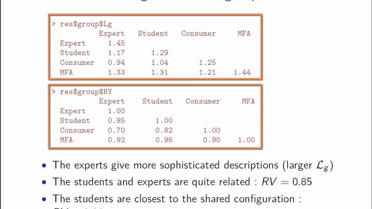
We saw in the previous video that MFRA is a specifically weighted PCA that provides an individuals plot and a variables plot entirely equivalent to those obtained with PCA. Let's now have a look at what the group structure in MFRA brings to the table. To begin with, we'll see how to obtain a certain representation of the groups of variables that will allow to globally compare the information provided by each group. Then, we will use the common framework provided by MFA to compare the results of the PCAs constructed from the data of each group. This means comparing the point clouds of individuals from one PCA to the other, and then the dimensions of the separate PCAs. First, let's go back to the construction of the principal components. In PCA, the first principal component is the variable with norm 1, which we call v_1 here, belonging to the space R^i which is most related to all of the variables, with most linked meaning in terms of squared covariance. If the PCA is normalized, the first component corresponds to the most related variable in terms of the squared correlation coefficient. As the MFA is a PCA on a weighted table, we can write the previous criterion in a way that shows the weighting used by MFA. Each variable x_k is divided by the square root of the first eigenvalue of the group to which it belongs. We have to sum over all the variables, but since the variables are organized in groups, we can write the criterion by making a sum over the group appear, and a sum over all the variables of the j-th group. We can extract the first eigenvalue lambda_1_j, And show that the first component of the MFA is the variable with norm one, which maximizes the squared covariance with the variables of all the groups, with the covariance being divided by the maximum axial inertia of each group. The maximum axial inertia corresponds to the inertia of the group's strongest axes. If lg of KJV one is the term in red, this coefficient. Lg of Kj, V1 corresponds to the projected inertia of all the variables of the jth group onto the variable V1. It is a measure of the connection between a group of variables and a variable. There is another well-known measure of the relationship between a variable and a group of variables, known as the R-squared, which is used in regression. The interest in Lg is that it is based on the inertia And in factor analysis, we always try to maximize inertia. The formula tells us that the first component of the MFA is the variable that maximizes the link with all the groups in the LG sense. In order to find the second principal component of the MFA, we must look for, among the variables orthogonal to the variable v1, the variable that is most linked to the whole set of groups according to the LG criterion. And so on for the following principal components. The coefficient lg varies between 0 and 1. It is equal to 0 if all the variables of the jth group are not correlated with the variable v_1. It is 1 if the variable v_1 is the same as the first principal component of the group. Indeed, the first principal component of the group is, by definition, the variable most linked to all the variables in the group, and thus maximizes the sum of the squared covariances. This sum of the squared covariances is equal to the inertia of the first principal component, which is the first eigenvalue of the group. Since the variables are weighted by the first eigenvalue of the group, the maximum L_G corresponds to the value 1. This L_G that we have just defined makes it possible to quantify the link between a variable and a group of variables. This measure can therefore be used to quantify the link between a group of variables and a principal component. This suggests that we can use this measure to construct a graph of the groups. A given group will have on the x-axis the coefficient L_G between this group and the first component, and on the y-axis the coefficient L_G with the second component. In our example, the representation of the groups in relation to the principal components of the MFA is as follows. We can see that all the juries have an x-axis value close to 1, and therefore a high LG with the first dimension of the MFA. However, a high LG means that the dimension of the MFA is linked to a strong dimension of the group, the first dimension, or one almost as large as the first one. Thus, in our example, the first dimension of the MFA is present in all groups, so it is one that's common to all groups. We can also see that the second dimension is much more linked to the expert group than to the other groups. This is not really surprising since we saw that the expert group had a larger second eigenvalue relative to its first eigenvalue than the other 2 groups. Lastly, the points representing the student and consumer groups are close to each other, which means that these groups have several dimensions in common and thus induce more or less the same structure on the individuals. This visual view of the data provides a kind of summary representation of the groups, and it's very easy to see which groups are broadly similar. 2 groups are similar if they are close on all the dimensions, but since the first dimensions summarize most of the information, it is often enough to compare the groups over the first few— 3 or 4 are generally sufficient. This graph makes it possible to globally compare the groups and therefore to see if the distances between individuals are similar from one group to another. In other words, if the point cloud seen by one group of variables and another group of variables are similar. We have defined the measure Lg between a component and a group of variables, but this measure Lg can be extended very easily to the connection between 2 groups of variables. We just have to calculate the sum of all the covariances between the variables of one group and the variables of the other. The variables being of course weighted by the weighting in the MFA. If we calculate the coefficient L_G between a group and itself, this amounts to calculating the dimensionality of this group by rewriting the criterion: the ratios of the squared eigenvalues of each component divided by the largest squared eigenvalue of the group. Appear. If the first eigenvalue is, is much larger than the others, then L_G will be close to 1 and the group is almost 1-dimensional. On the contrary, if many eigenvalues are close to the value of the first eigenvalue of the group, then several dimensions of variability are important and the group will be multidimensional. This coefficient can thus be seen as a dimensionality indicator for a group. Lastly, the disadvantage of calculating the coefficient Lg between 2 groups is that this criterion is not bounded. If instead this Lg between 2 groups is normalized by the dimensionality of each of the groups, what we get is called the RV coefficient. This RV coefficient varies between 0 and 1, and it is easier to use to know if 2 groups are linked or not since it's bounded by 1. However, this coefficient tends to be larger when the number of individuals is small or when the number of variables in each group is large. Coming back to our example, the LG and the RV between the groups are as follows. As the matrix is symmetric, we show here only the lower diagonal terms. From the LG, it can be seen that the expert jury gives a more multidimensional description and thus richer of the wines than the other juries because the LG is higher. If we look at the RV coefficients, we see that the student and expert juries are close to each other because the RV is close to 1, 0.85. Lastly, we can consider the mean configuration of the MFA and look at the link between this and each group. The mean configuration of the MFA is here a group corresponding to the set of coordinates of the individuals on all the dimensions. It is the shared or mean configuration. These RV coefficients are given in the MFA row. We can see that the student jury has a configuration that is very close to the mean one since the RV is close to 1. It's 0.96. Let's now look at another way of comparing the groups starting from the configurations of individuals in each group. For this, the typologies provided by each group will be compared in a shared framework, more precisely in the shared reference frame given by the MFA. Comparing the typologies means asking if individuals are seen in the same way by the different groups or if certain individuals are specific to some groups. To do this, we will proceed as follows. Let's illustrate the approach with a dataset containing 3 groups of variables. The MFA is first built from these 3 groups as we have seen earlier. This gives us a representation of the individuals on the principal dimensions of the MFA. The individuals are in a space R^k with k dimensions where this space is the direct sum of the spaces R^kj generated by each group of variables. Let's now try to represent each individual in the dataset using only the data from one group of variables. We will call partial individual i to the power of j the ith individual seen by only the variables in group j. How can we represent this partial individual? And above all, how can we represent all of the partial individuals associated with the ith individual? Namely the partial individuals i1, i2, up to iJ in the same plot. The shared plot is the space provided by the MFA using data from all of the groups. We juxtapose one table per group with the main data table. In the subtable for group j to be projected, all variables that do not belong to group j take the value 0 because the array is centered and otherwise the values would be the means of the variables. Also, the values of the variables belonging to group j are centered and possibly standardized if we have standardized the variables of this group, and divided by the square root of the first eigenvalue of the group. In other words, the values used in the overall MFA analysis. These partial individuals are then used as supplementary individuals and thus projected onto the axes of the global analysis. We thus get the projection of the ith individual seen by the variables of group 1, shown here in red. An important point, however, is that since we have 0 for all groups other than group 1, the partial point of group 1 tends to be found near the center of the point cloud. This is true for all partial individuals in each group. To be clear about this, let's take the trivial example where the 3 groups of variables are identical. All the partial points of the same individual should be superimposed and also superimposed on the average individual. Now, if we calculate the projection of a partial individual of a group, as it takes the value 0 on the other 2 groups, its coordinates will be close to the point cloud's barycenter. It will in fact be 3 times too close to the barycenter. Thus, the projection of all the partial points must be dilated by a factor of 3 in our example. When the dataset has J groups, the partial points must be projected as supplementary points and then dilated by a factor of J. With this dilation, we have for each individual as many partial points as there are groups, and the mean point corresponding to the individual seen in the global analysis is at the barycenter of the partial points. The partial points representation is therefore very useful since it makes it possible to compare the representation of individuals from one group to another. Take the following example. Individuals were first questioned on several issues related to their opinions. Then, they were interviewed on several issues related to their behavior. These 2 sets of questions can be considered as 2 sets of variables in the MFA. The MFA then provides a representation of the individuals as seen by all of the variables. This means the point corresponding to the global analysis, that is the mean point here in purple. An interpretation of the positions of the mean points on the dimensions can be made as is done in PCA. We can also represent the partial points corresponding to an individual seen only in terms of the opinion variables and then only in terms of the behavioral variables. If the 2 partial points are close to each other, and therefore close to the mean point, then the individual behaves in accordance with their own opinions, whereas if the partial points are far apart, then the individual doesn't behave in accordance with their own opinions. The distance between the 2 partial points is a way of visualizing this discordance. Let's take another example involving a questionnaire which participants in a course answered before starting the course. Several questions relate to their expectations of the course. A second questionnaire was sent to the same people at the end of the course. The questions in it relate to what the participants have learned during the course. The individual on the right has its 2 partial points close together, while the individual on the left has them far apart. The individual on the right therefore got from the course what they expected from it, So, we can suppose that they were satisfied. The individuals on the left, on the other hand, didn't learn what they expected to learn from the course. You could even say that they were surprised by the course. But what type of surprise? In other words, were they disappointed? Or were they surprised but in a good way? To find out, we can return to the interpretation of the dimensions and, more specifically here, to the interpretation of the first dimension which separates the 2 partial points. If positive coordinates on the axes are related to a strong positive appreciation, then the individual has learned more than they expected from the course and can be said to have been pleasantly surprised. And if not, we can suppose that they were disappointed. This shows that the position of the mean points, that is, of the individuals seen by all of the variables, and the positions of the partial points can be interpreted using just a single plot of the shared dimensions of the MFA. The transition formulas that we have seen in PCA can be directly applied to the mean point in the MFA. Remember that these transition formulas make it possible to interpret an individual's position thanks to the variables plots. An individual is to be found on the side of the variables for which they have large values and opposite from variables for which they have small values. These transition formulas can also be used for the partial points. We just have to restrict the relevant formula to the variables of group j. As mentioned earlier, we multiply the coordinates of the partial points by j, the number of groups, so that the coordinates of the partial points and the mean points can be interpreted all at once and on the same scale. The dilation by a factor j applied to all the partial points puts the mean point at the barycenter of its partial points so that mean and partial points are represented on the same scale. In our wine example, this superimposed representation looks as follows. The points in black correspond to the wines as seen by all the juries. The points in color correspond to the partial points. In red, the wines seen only by the expert jury, in green by only the student jury, and in blue by only the jury of consumers. Each black dot corresponding to the mean wine is of course at the barycenter of the colored points. We can see that all the wines are interpreted fairly homogeneously by the 3 sensory juries because all the partial points for each given wine are close to the mean point. Except perhaps the Aubusière Select wine, lower left, which was perceived as more extreme by consumers than by experts for variables related to the first dimension. Indeed, on this dimension, the value for this wine is strongly negative for consumers and fairly close to 0 for the experts. Visually, we can see that the coordinates of the partial points are relatively similar from one group to another for the first 2 dimensions. In fact, we can define an index measure to quickly and globally calculate whether the coordinates of the partial points are close to those of the mean point axis by axis. To do this, for a given axis, we are going to break down the total inertia of the partial points. For the S dimension, the total inertia of the partial points can be broken down into the mean between-points inertia, that is between individuals, and the within-individual inertia. Also, we can calculate the ratio of the between-points inertia to the total inertia. In our example, for the first dimension, the ratio is 0.93 and is therefore very close to 1, which means that the coordinates of the partial points with respect to a given individual are very close to each other and therefore very close to the coordinates of the corresponding mean point. The within-inertia, which measures the similarity between partial point clouds dimension by dimension, can also be broken down by individual. This decomposition by individual is very useful for sorting individuals in terms of decreasing within-individual inertia and for identifying which individuals are perceived differently by each group of variables. When interpreting differences between groups, these individuals can be examined more closely. We have compared the groups of variables using the partial points plot, which represents the features of the individuals of each of the groups in shared global space. It is also possible to compare groups using the dimensions of separate analyses, in other words by comparing the principal components of the PCAs for each group. To do this, we are going to take a closer look at the principal components of the PCA of a given group. And in fact, we are going to use them like supplementary variables in the global analysis, that is in the MFA. This will allow us to project the principal components of this group and see how these components are related to the MFA axes. If the principal components of the group are highly correlated with the dimensions of the MFA, then the individual plots in the PCA of this group will have the same form as the individual plots of the mean points of the MFA. For our example, here is the plot which gives the projections of the principal components of the individual PCA onto the first 2 dimensions of the MFA. The first dimension of the students PCA is highly correlated with the first dimension of the MFA. Therefore, wines with a small coordinate value or a large one on the x-axis of the PCA for the students data have a small coordinate value or a large one on the x-axis of the MFA. The same is true for the second dimension of the students PCA which is also highly correlated with the second dimension of the MFA. This means that the description of the wines provided by the students is very similar to the description of the wines obtained by the MFA, and therefore that of all of the juries. For the experts, dimensions 1 and 2 of the PCA do not exactly coincide with dimensions 1 and 2 of the MFA. However, the PCA dimensions are both well projected, which means that The PCA's first-second dimensions built using the expert data is close to the MFA's first-second dimensions but with a rotation. The same thing has happened with the consumer's data.