PCA (course 2/3): interpretation of the graph of individuals and variables
In this instructional lecture, the presenter walks through the practical steps of applying Principal Component Analysis (PCA) to high‑dimensional data. Beginning with the geometric view of individuals as points in a K‑dimensional space, the talk explains how similarity is defined via Euclidean distance, and why centering and (optionally) standardizing variables are essential preprocessing steps. The concept of inertia (the multivariate analogue of variance) is introduced as the criterion for selecting optimal low‑dimensional viewpoints that preserve the shape of the point cloud. The speaker details how PCA finds successive orthogonal axes that maximize projected inertia, linking this to singular value decomposition and eigen‑decomposition of the correlation matrix, and interprets eigenvalues as explained variance. Using a wine sensory dataset (10 wines × 27 attributes), the lecture demonstrates how to read individuals plots (scores) and variable plots (loadings) – the correlation circle – and how the cosine of angles between variable arrows reflects their correlations. Duality relationships between the individuals and variables clouds are explained via transition formulas, and the importance of projection quality (well‑represented variables lie on the unit circle) is highlighted. Throughout, visual analogies (flocks of starlings, 3‑D teapot, camel) illustrate viewpoint selection and the trade‑off between dimensionality reduction and distortion. The session concludes with a summary of how PCA simultaneously provides an optimal representation of both individuals and variables, enabling meaningful interpretation of the main sources of variability in the data.
Chapters
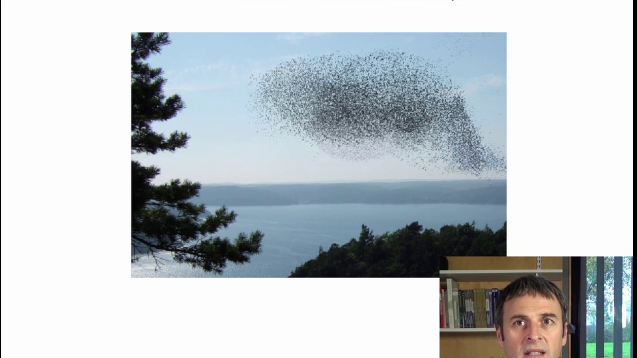
Now that we have defined the types of data we can do PCA on, and what kinds of questions we can examine with PCA, let's now see how to put PCA into practice. We said that an individual is a row of the data table, and therefore a point in K-dimensional space. If K is equal to 1, there is only 1 dimension, and it is easy to represent the individuals. I put them on a 1-dimensional line according to their value. If there are 2 variables, I can put them on a standard scatter plot like we can do before linear regression. If there are 3 variables, it becomes a little more difficult, but there are softwares that can show datasets in 3 dimensions. The software can help visualize a point cloud by pivoting the axes in various directions, thus giving us a better feel for where the point cloud is. But if there are 4 variables or more than 4, it is impossible to represent a point cloud in this many dimensions. However, the mathematical concept behind it is simple and stays the same: there are k coordinates for k dimensions. So how are we going to be able to look at the cloud of individuals if it exists in a very high-dimensional space? Well, we can start by defining a notion of similarity between pairs of individuals. When can we say that 2 individuals are similar? How about— 2 individuals are similar if they are close. If so, we can calculate the squared distance between individuals, thanks to Pythagoras, by the sum of the squared differences between each variable for the 2 individuals. This is a simple definition of similarity. So finally, when I say I want to study the cloud of individuals, This just means studying the shape of this cloud to see which individuals are close to each other or far apart. The data table can be studied geometrically via the distances between individuals. And this turns out to mean studying the shape of the point cloud. We can see in the photograph a flock of starlings. The cloud of birds exists in 3 dimensions, but the photo allows us to visualize it in a lower-dimensional space here 2 dimensions. This 2D representation nevertheless gives us a good idea of the cloud's shape in the original 3D space and thus a good idea of the distances between birds. The moral of the story is: when our individuals exist in a high-dimensional space, we will try to study the shape of the cloud and visualize it in 2 dimensions. To study the cloud's shape, we first have to mention centering and standardization. Centering data means translating the cloud of points so that its center of gravity ends up at the origin. The cloud's shape remains the same when translated. Centered data gives technical advantages and is always done in PCA. Next, we can consider whether or not to standardize the data. In the graph on the right, we have a representation of individuals in terms of size and weight. The size is in centimeters and the weight in quintals. Note that the data are centered here. We can see that the point cloud is very elongated and vertical. In the middle graph, the size is in meters and the weight in kilograms. The shape of the cloud is quite different from the first one. We now have a very elongated horizontal point cloud. And as we said, we want to study the shape of the point cloud. But depending on the units chosen, quintal and centimeters or meters and kilograms, the cloud shapes can be very different. How can we handle this? One idea is to standardize the data. If we standardize our variables, they then have no units and are therefore comparable. This type of data standardization is essential if measurement units are different from one variable to the next. If the variables are already in the same units, we can choose to standardize or not. We will see later that standardizing leads to giving the same importance to each variable. Without it, the bigger the variance, the more important a variable is. It is not obvious in this case whether to standardize or not. In our example in the course, we will standardize the dataset. The standardized dataset already provides some useful information. For instance, we see that the abuse domain wine has a very low score for bitterness and aroma intensity. Values below -2 are below the average for that variable, and indeed quite extreme. We know that when values are from a normal distribution, they are between -1.96 and 1.96 95% of the time. Here, it is not necessarily the case that the data follow a normal distribution, but a standardized value below -2 is still very extreme. So the Buisse Domain wine is especially not bitter with very low aroma intensity. The wine V, Aubusier Select, is rather sweet and non-acidic. Our method, principal component analysis, will then be used to analyze this standardized data table. This means that we want to visualize it. It is difficult to visualize this table since there are 27 variables. As it is not humanly possible to visualize 27 dimensions, We aim to get an approximate look at the cloud of wines from a good viewpoint in a low-dimensional space. For such a representation to be successful, it must select a good viewpoint. In fact, PCA turns out to mean searching for the best smaller space, lower-dimensional, that gives an optimal view of the k-dimensional cloud's shape. We often work in a plane, though this can prove inadequate when dealing with particularly complex data. So, what is a good viewpoint? It's one that lets us get an idea of the distance between individuals in a way that it distorts the higher-dimensional truth as little as possible. That is, the viewpoint should maintain the point cloud shape as closely as possible. Here is a 3D animation to help us think about the question. Here is the point cloud in 3 dimensions. I can move the point cloud to see it better. This gives us an idea of what the point cloud really looks like in 3 dimensions. Then it's possible to only have a 2D representation of the 3D point cloud. This is the first suggestion for a 2D viewpoint. Here is a second. And a third. And so the question is, among these 3 possibilities, which one should you choose to get the best understanding of the point cloud? We are only allowed to have a single photograph of the 3D cloud Which one should we choose? Well, I would intuitively choose the 3rd one. Why? Because it spreads out the points. It seems to better see the distances between individuals. And this intuition is good. So viewpoint quality means the quality of reproduction of the cloud's shape. A viewpoint is good if we can see the diversity and variability in the data and is especially good if it does not overly distort distances between individuals. The true distances are calculated between individuals in a high-dimensional space, and now we have put them into a 2D space. This modifies the distances between individuals, and we want these distances to be as little modified as possible. So how can we quantify a viewpoint's quality? The answer is with the concept of dispersion. A point cloud can be best seen if its projection onto a 2D plane is spread out, if we can see a lot of variability. This variability exists across several dimensions and is called inertia. Thus, we will talk about inertia from now on. Inertia is simply a generalization of variance to several dimensions. Here is another small illustration, again a visualization of a 3D cloud. Here I have a picture of an animal that lives in a 3D space, but I have a photo of it that's only in 2D. So which is the photograph that best reproduces the shape of my cloud in the original space? It would seem to be the one on the right. I can see the camel the best because I can see more information and in particular 2 humps and 4 legs. If we go deeper into the details, how can we find the best approximate viewpoint of the cloud? Well, we begin by finding the first component, also known as the first axis, that distorts the cloud as little as possible. Let us denote h_i the projection of individual i onto an axis, and O the center of gravity of the cloud. Then, I_Hi squared is the squared distance between the individual in the cloud and its projection onto the axes. And what we want is that the squared distance between an individual and its projection be as small as possible. Since the distance O_i between an individual and the origin is always the same, I_Hi is small if O_Hi is large, Thanks to Pythagoras. So, since O_i squared is constant, I_h_i squared is small if O_h_i squared is large. So, we want O_h_i squared to be as large as possible. Since we want each O_h_i squared to be as large as possible, we really want the sum of the O_h_i squared to be as large as possible. And the sum of the O_h_i squared is none other than the dispersion of the projected points, That is, we want these projected points to be as spread out as possible. This is how we find the first PCA axis, also named the first PCA dimension. Let's now consider what it means to find the best viewpoint of the cloud in 2 dimensions. Now, the cloud is projected onto a plane, also chosen to minimize distortion of the point cloud. The plane is selected so that the distances between the projected points on the plane H_i— H_i is now the projection onto the plane— are as close as possible to the distances between the initial points. Since in projections distances can only decrease, we can try to make the projected distances as large as possible. So once again, we want the sum of the O_H_i squared to be as large as possible. What is quite nice is that the best plane in 2D contains the best component in 1D. So to find the best plane in 2D, you don't have to start from scratch. You can simply find the first PCA dimension, then look only at orthogonal directions to the first one, and find that which maximizes the sum of the OHi squared. In the same way, once we have found the second dimension, we can find the third, and so on sequentially. So each new axis is orthogonal to all previous ones and maximizes the inertia. From a technical point of view, PCA axes are obtained by a singular value decomposition or by diagonalizing the correlation matrix to extract the eigenvectors and eigenvalues. The eigenvectors are vectors u_s associated with the eigenvalue of rank s. The eigenvalues are ranked in decreasing order. The eigenvalue lambda_s can be interpreted as the inertia of the cloud projected onto the s-th component. In other words, lambda_s corresponds to the explained variance for the component of rank s. We can visualize this with a small illustration. Here we have a teapot in 3 dimensions, and we want to find the best direction in which to visualize it from just one viewpoint. Well, to start, we find the first axis. Here is the one that allows us to best see the teapot. So if we had to project the teapot's points into one dimension, we would choose a red dimension. And now we want a second axis, orthogonal to the first. We have defined the first, so now we find such an orthogonal axis to it. This gives us the second axis, in green. Let's now look at the wine dataset with the 10 wines and 27 sensory attributes, 2 preference variables, and the qualitative variable corresponding to the wine labels. We want to characterize the wines from a sensorial point of view, so first we just consider the 27 quantitative sensory variables. Well, if we plot the individuals using PCA, we get this graph. It shows, for instance, that S. Michaud and S. Trotignon are very close. What does it mean when I say S. Michaud and S. Trotignon are very close? It really means that the scores for Es Michaud and Es Trottignon are approximately the same whatever the variable. The scores are almost the same, so the points are close. In the same way, Aubusier Marnier and Fontenay Coteaux are wines with similar sensory scores for the 27 attributes. On the other hand, Fontenay-Brûlés and Es Trottignon have very different sensory profiles because the first principal component, representing the main axis of variability between wines, separates them strongly. Since these wines are far apart in the first dimension, they must be very different because the first dimension is that which separates the points as much as possible. So then, why are these 2 wines so far apart in the first dimension? To answer this, it might help to be a French wine expert. I personally am not. So we have to use the variables we have to interpret the dimensions. What are the differences between Font Brûlé and Estrottignon? To answer this, we can look at the individual's coordinates in each dimension. For instance, Aubusière-Silex has a value of 1.1 in the first dimension. Let's call this value fi1, 1 for the first dimension. Similarly, we have fi2 in the second dimension, which equals -6. So, for each individual i, we consider its values on the horizontal and vertical axes. Thus, we can create 2 vectors, one which gives the values for all individuals in the first dimension, the other that does the same in the second dimension. Therefore, these vectors have i entries, the same number as there are individuals. Then, in order to interpret the plot for the individuals, we will calculate the correlation between each variable, for example vanilla odor, and the first dimension. So we do this, and then calculate the correlation between vanilla odor and the second dimension. If this odor is related to the first dimension, it means that its values are related to the coordinates in this dimension. Thus, if the correlation is close to 1, it means that individuals who have small values for vanilla odor have small values in the first dimension. And thus, such points will be to the left of the plot. And individuals who have large values for vanilla odor will have large values in the first dimension and will be found to the right. If the correlation is negative, it means that individuals with small values in the first dimension have high values for vanilla odor, and that individuals with large values in the first dimension have small values for vanilla odor. The same logic applies in the second dimension. Using this information, we can build a graph that represents all the variables. They will all be found inside a circle known as the correlation circle. In our example, the graph of the correlation circle shows that: The variables astringency, visual intensity, mushroom odor, and candied fruit odor found to the right have correlations close to 1 with the first dimension. Since the correlation with the first dimension is close to 1, the values of these variables move in the same direction as the coordinates in the first dimension. Wines with a small value in the first dimension have low values for these variables. And wines with large values in the first dimension have high values for these variables. Thus, the wines that are to the right of the plot have high and positive values in the first dimension and thus have high values for these variables. With the same logic, wines that are to the left have a small value in the first dimension and thus low values for these variables. For the variables passion fruit odor, citrus odor, and freshness, everything is the other way around. The correlation with the first dimension is close to -1, and thus the values move in the opposite direction. Wines with a low value in the first dimension have low coordinate values, and thus have high values for these variables. And wines with large values in the first dimension have small values for these variables. Overall, we see that the first dimension splits apart wines that are considered fruity and flowery, on the left, from wines that are woody or with vegetal odors. And this is the main source of variability. So then, how can we interpret the second dimension, the vertical axis? At the top, wines have large values on the vertical axis. Since the correlation coefficients between the 2nd dimension and variables such acidity or bitterness are close to 1, it means that wines at the top take large values for these variables, and wines at the bottom have small values in the 2nd dimension and thus small values for these variables. For sweetness, the correlation coefficient is close to -1. So wines that have a small value in the second dimension are sweet, while wines that have large values are not. Overall, the second dimension separates the wines at the top, acidic and bitter, from sweet wines at the bottom. So for our data, the main direction of variation involves odor, and the second separates sweet wines from from acidic and bitter wines. Let's now take a closer look at the variables. Well, a variable is a point in an high-dimensional space since each variable has high values, one per individual. So we can consider the variables cloud that lives in a high-dimensional space. Variables are represented by arrows in principal component analysis. So variable k is an arrow from the origin The cosine of the angle theta_k,l between the arrows for variables l and k is equal to the scalar product of the variable k with the variable l divided by the norm of variable k times the norm of variable l. This is equal to the sum over all i of x_i,k times x_i,l divided by the square root of the sum of the squares of the x_i,k times the sum of the squares of the x_i,l. As the data matrix X is centered, we can actually look at this formula as the sum of the Xik minus the mean of Xk times Xil minus the mean of Xl divided by the standard deviation of the variable k times the standard deviation of the variable l. Which means that when the data are centered, we see that we are looking at the well-known correlation coefficient between 2 variables. So we have here a geometric representation of the correlation coefficient between 2 variables K and L. The geometric representation of the correlation is none other than the cosine of the angle between variables K and L. If the variables have been standardized, the lengths of arrows in this space equal 1, and all arrows will have their tip on the surface of an i-sphere of radius 1. So for each variable, we have an arrow from the center of the i-sphere that reaches the i-sphere of radius 1. The question now is, how can we actually see the variables cloud? It's in an i-dimensional space, and humans can't visualize that easily when i is 4 or more. Well, what we can do is look for directions from which we can see the variables cloud as well as possible. So it's the same trick as for individuals: we look for orthogonal axes that best represent the variables. The first dimension, the one that lets us see the variables the best, will maximize the sum of the correlations between that dimension's direction and each variable. So, the best axis V1 is that which is the most related to all the variables, in terms of the squared correlation coefficient. So, essentially, V1 is like a synthetic variable that best summarizes all variables. Once we have the first axis, we can find a second one, orthogonal to the first, which is the next most linked to the variables. This second dimension contains information not found in the first. Once we have found it, we can sequentially find the third dimension, and so on. So what happens when we fit the variables for our dataset in this way? We find the same representation as before. Earlier, we had built a representation of the variables to help us interpret the individuals' point clouds. And then, when we built the best representation to see the variables' clouds, we find the same thing. So that's a little magic. Amazing! So in summary, this representation helps us interpret the individuals' point clouds to characterize individuals. In our example, this means dividing them into fruity and flowery wines, sweet wines, acidic and bitter wines. It is also, as we have seen here, an optimal representation of the variables cloud. And we also get to visualize all the correlations between pairs of variables by the cosine of the angle between them. So this representation is also a way to visualize the correlation matrix. What is magical is that it's the same thing! The relationships between the individuals' and variables' point clouds are called duality relationships. This term refers to the dual approach to the one single data table by considering it either by row or column. This approach also involves transition formulas that let us calculate the coordinates in one space from those in the other. Let us note FIS the coordinates of individual i and GKS the coordinates of variable k in the rank s component or dimension. The vectors f.S are called the scores and the vectors g.S divided by the square root of the S eigenvalue are called the loadings. The transition formulas are the 2 following relationships: give an individual's coordinates using the data and the variable's coordinates, and second, give a variable's coordinates using the data and the individual's coordinates. This result is very important for data interpretation and makes PCA a rich and reliable experimental tool. What we find is: individuals are found on the same side as their variables with high values and opposite their variables with low values. Remember also that the x_ik are centered and have both positive and negative values. This is one reason why individuals can be so far from variables for which they have small values. For instance, the variable sweetness has a low value in the 2nd dimension and the value of Aubusière Silex for sweetness is high. Thus, the multiplication gives a negative value which contributes to the fact that the value of Aubusière Silex is low in the 2nd dimension. The value for acidity is high in the 2nd dimension and Aubusière Silex has low acidity less than the mean, so the positive value for acidity multiplied by this negative value for Aubusière silex gives a negative value. This contributes to the fact that the value for Aubusière silex is low in the 2nd dimension. It is exactly the same reasoning for the variables. Now, let's go back to the graphical view of the variables. We have seen that the correlation coefficient between variable A and variable B is equal to the cosine of the angle between them. However, this is in the high-dimensional space, and we are visualizing it in the projected 2D space. So, here is an illustration that allows us to see the scatter plot of the variables on the left and their projections on the right. For example, variables D and E point very close to the projection plane. The projection of D, called HD, is very close to D because the D is close to the projection plane. This is the same for HE, which is close to E. So the angle between D and E is very close to the angle between HD and HE. And therefore, the angle in the projection plane can indeed be used to visualize the correlation between D and E. More precisely, the cosine of the angle HDHE is almost the same as the cosine of the angle between E and D, because the variables are well projected. On the contrary, when variables are not well projected, which is the case, for example, for A and B, the angle in the projection plane is small, while that in the original space is very large. The arrow A takes a large value in the third dimension, while B takes a small one. So these 2 arrows are approximately projected to the same place, but poorly. Therefore, the cosine of the angle here is nowhere near the cosine of the angle in the original space, and therefore we can't really get the correlation coefficient between A and B. The cosine of the angle we see is nowhere near the correlation coefficient. Our conclusion is: you can get a feel for the correlation coefficients only for well-projected variables, that is, variables pointing close to the correlation circle. Indeed, what we have in general is an i-sphere of radius 1 cut by a plane. Thus, the i-sphere is projected onto a circle of radius 1. If 2 arrows are close to the edge of the circle, their variables are well represented and we can visualize the angle between them in the global space. On the contrary, it is impossible with only the projection to have an idea of the correlation coefficient between 2 poorly represented variables like A and B in our example. So basically, we can only really interpret well-represented variables. We have seen how to construct plots of individuals and variables. We will see in the next video some useful interpretation aids which will be of great use for finishing up a PCA analysis.
More from Yamossoun











Algorithme de calcule de la racine carrée par dichotomie #dichotomy #squareroot #algorithm