The lecture presents a suite of practical tools for interpreting the results of a Principal Component Analysis (PCA) and for incorporating categorical (qualitative) variables into the interpretation. It begins by explaining how the percentage of inertia (explained variance) associated with each principal component can be visualized with bar charts, used to decide how many dimensions to retain, and compared against reference tables or cross‑validation (estim_ncp). The speaker then distinguishes active elements (variables and individuals that define the components) from supplementary (illustrative) elements, showing how supplementary quantitative variables are projected as correlations and how supplementary qualitative variables are represented by category centroids. The concept of quality of representation (cos²) for both variables and individuals is introduced, together with the calculation of contributions (percentage of squared correlations) that highlight which variables or individuals drive a given dimension. Automated characterization methods are described: ranking quantitative variables by absolute correlation with a component, and for categorical variables performing one‑way ANOVA and Student t‑tests to assess association with component scores, sorting by p‑values and correlation ratios. The speaker outlines a step‑by‑step practical workflow: selecting active vs supplementary variables, deciding on standardization, running the PCA, choosing the number of dimensions, interpreting plots while checking cos² and contributions, and validating any inferred similarities against the raw data. Finally, resources are provided, notably the FactoMineR R package, recommended textbooks, and additional video tutorials. The overall message is that careful quantitative diagnostics and the inclusion of supplementary categorical information greatly enrich PCA interpretation.
Chapters
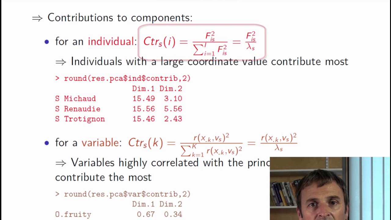
In the earlier video, we have seen how to construct plots of individuals and variables. Let's now take a look at some useful interpretation aids which will be of great use for finishing up a PCA analysis. We have seen that what helps an interpretation is the quality of the projection. This can be measured by the percentage of inertia explained by the 1D or 2D mapping. This percentage can be seen as the percentage of the overall information contained in the 1D or 2D mapping. We can plot a bar chart with the percentage of variance, or percentage of inertia, explained by each dimension. So here, we see that the percentage of explained variance in the first dimension is approximately 43%, and around 25% in the second. Together, the 2 dimensions explain 68% of the information contained in the dataset. These percentages are displayed on the graphs of individuals and variables. This is what is written here: 43% of the information on the first dimension, 25% on the second. So initially there were 27 variables and we summarized them in 2 dimensions containing 68% of their information. So we get a fairly good summary of them. But then, in the next dimensions, there is less and less information. This bar chart is useful for choosing the number of dimensions that should be used for interpretation. We look for a visible jump or gap in the bar chart. There are also tests for selecting the number of dimensions, or even cross-validation can be used. The function estim_ncp performs cross-validation. We can also see PCA as a denoising method that separates the signal found in the first dimensions from noise in later dimensions. This is a bit beyond the scope of the course, but PCA can be used for preprocessing before clustering, for instance. Now, here is a table which gives us the 95th percentile of the percentage of inertia found in the first 2 PCA dimensions. When we have independent variables. So, for example, with 15 individuals and 12 variables, the value 47.8 tells us that, having performed 10,000 PCA with 15 individuals and 12 independent variables, we have calculated the percentage of variance found in the first 2 dimensions, and 95% of these values are less than 47.8. Here is another table where the number of variables is greater. With 10 individuals and 27 variables, the 95% quantile of the percentage of inertia is approximately 43%. In our example, we had a value of 68%, which is higher than 43%. So our plane explains more information than a PCA plane would have with independent variables. This means that our summary is very concise and that we don't only have independent variables. There must be strong relationships in our dataset. Here are some more aids for interpreting results if we have access to supplementary variables or individuals. What we call active elements are individuals and variables used to build the principal components. So supplementary elements or illustrative elements are extra individuals or variables that have not been used to build the principal components. They can be used instead to illustrate or further interpret the PCA. Illustrative elements can be quantitative variables, qualitative variables, or individuals. By definition, supplementary quantitative variables play no role in calculating distances between individuals. They can be represented in the same way as active variables to hopefully assist in interpreting the individual's point cloud. The value of a supplementary variable in a given dimension corresponds to the correlation coefficient between the variable and the principal component. Supplementary variables can therefore be represented on the same plot as active variables. In our example, we see that the overall appreciation variables are not strongly linked to the sensory attributes since they are not well projected onto the first 2 dimensions. For supplementary qualitative variables, we can project the center of gravity of individuals from each category. For the label variable, with categories Sauvignon and Vouvray, we put Sauvignon at the center of gravity of the 5 Sauvignon wines and Vouvray at the center of gravity of the 5 Vouvray wines. Note that the qualitative variable is represented on the plot of the individuals, not on that of the variables. If we have several qualitative variables, we can calculate the centers of gravity for each category of each qualitative variable. Another indicator useful for interpretation is the quality of the representation. We can look at the quality of representation of a variable or individual. The quality of representation of a variable is measured by the squared cosine of the angle between it and its projection onto the plane or axes. Similarly, the quality of representation of an individual is the squared cosine of the angle between the vector from the cloud's center of gravity to the point i corresponding to the individual and the vector from the cloud's center of gravity to the projected point h_i. The cosine is calculated dimension by dimension, so we see for example that for Renaudie, the cosine squared with the first dimension is 0.73 and 0.15 with the second. Thus, to define the quality of projection onto the plane, we sum 0.73 0.15 0.88. This means that the angle is close to 0, and therefore this individual is well projected. We can thus allow ourselves to interpret the distance between this individual and other well-projected individuals. However, if 2 individuals are close to each other on the plane but poorly projected, we should not be quick to interpret their proximity because they may be far apart in the other dimension. As for the variables, passion fruit odor is well projected, whereas fruit odor is poorly projected onto the first 2 dimensions. Another thing we can look at is a variable's or individual's contribution to the construction of a given dimension. A variable's contribution is just the square of the correlation coefficient between it and that dimension divided by the sum of squared correlations between all variables and that dimension. This will tell us whether there is some variable that contributes significantly to that dimension with respect to the others. Next, individuals. An individual's contribution is the square of its coordinate value on the dimension of interest divided by the sum of the squares of the coordinate values of all individuals. These contributions are expressed as percentages. Again, if some individual contributes significantly to a dimension, it means that this dimension is probably mainly due to that individual. And without this individual, the dimension would be quite different. If this happens, we can state that this individual is important and try to explain why. Then, it could be interesting to perform the analysis again without them to see if and how much the dimensions change to see if the first dimension of variation is still the same or if it is a bit different without this individual. Next, here are some tools that can help interpretation, especially when there are lots of variables. The components provided by PCA can be automatically characterized using all of the variables, whether quantitative or categorical, supplementary or active. For quantitative variables, the principle is the same whether they are active or supplementary. First, the correlation coefficients between the coordinates of the individuals on component s and each variable are calculated. We then sort the variables in descending order from highest to lowest coefficients and keep variables with highest correlation coefficients in absolute value. In our example, for the first dimension, we see that the most correlated variables are candied fruit odor and grade with correlations close to 1. These therefore best describe the first dimension. There are other variables which are highly positively correlated with the first dimension, and others that are highly negatively correlated with coefficients close to -1. For example, freshness, passion fruit odor, etc. So clearly, there are many variables that characterize the first dimension. There are, however, fewer that characterize the second. This is expected since the second dimension is less related to the variables than the first, by construction, since the first is the main direction of variation. We see that odor intensities are strongly positively related to the second dimension, and sweetness is fairly strongly negatively related. For categorical variables, we do one-way analysis of variance, that is one-way ANOVA, and seek to characterize the coordinates of individuals on component s in terms of the categorical variable. We use the constraint that the sum of the coefficients equals 0. Then, for each categorical variable, an F-test is performed to see if it is related to the given dimension. Second, a Student t-test is performed to compare the average of the individuals who have that category with the general average. We test whether the coefficient equals 0, supposing that the variances of the coordinates are equal for each category. The one-way ANOVA coefficients are sorted according to p-values, in descending order for the positive coefficients and ascending order for the negative ones. For our variable Label, the squared correlation ratio is 0.87, which means that 87% of the variance of the coordinates of individuals in the first dimension is explained by the variable Label. And also, this is significant. We see also that the Vouvray have significantly positive coordinates in the first dimension, whereas the Sauvignon have significantly negative ones. These tips for interpreting data are particularly useful for understanding components when we have a lot of variables. To conclude, how do we implement PCA in practice? First, we must choose which variables will be active, that is to say, which variables will be used to calculate the distances between individuals, and which variables will be kept aside as supplementary. These supplementary variables don't contribute to building the dimensions but may be used for interpreting them. Then, we must decide whether to standardize variables or not. Standardization is essential if the variables have different units. When they have the same units, both solutions are possible and lead to separate analyses. This decision is therefore crucial. Standardization means that every variable has the same importance. Not standardizing the data therefore means that each variable is weighted with a weight corresponding to its standard deviation. This choice is therefore all the more important if the variables have quite different variances. The next step is to perform the PCA. Then we have to choose the number of dimensions we want to interpret. Interpret the first 2 only, or also the 3rd and 4th? If we do go to 3 or 4, we now must extend the PCA to this many dimensions. Next, we interpret the PCA results using both the plots of the individuals and variables. We're going to go back and forth between these 2 plots, trying to quantify and understand the differences and similarities between individuals and the relationships between variables. We can use indicators to enrich our interpretation, for instance calculating contributions using the squared cosine to be sure that distances seen in the plane are representative of distances in the global space. And lastly, when we conclude that 2 individuals are similar, it is important to go back to the raw data to be sure that we have not misinterpreted things. Whenever the analysis suggests an interesting interpretation, we should return to the raw data or standardized data to validate what has been inferred. To conclude, here are some useful supplements to the course. There are many books on exploratory multivariate data analysis, and we suggest in particular the ones that follow the structure of this course. Exploratory Multivariate Analysis by Example Using R. There is also an R package called FactoMineR that lets you do PCA with supplementary quantitative and qualitative variables, with many indicators such as quality of interpretation, contribution, etc. And lastly, there are several videos on YouTube and a YouTube channel playlist with videos in French and English. Some of these videos show how to perform PCA without missing values, others how to handle missing values in PCA. You've now arrived at the end of the course videos for principal component analysis. Next, go and watch the video on how to use principal component analysis in practice using FactoMineR and have a go at the suggested exercises.