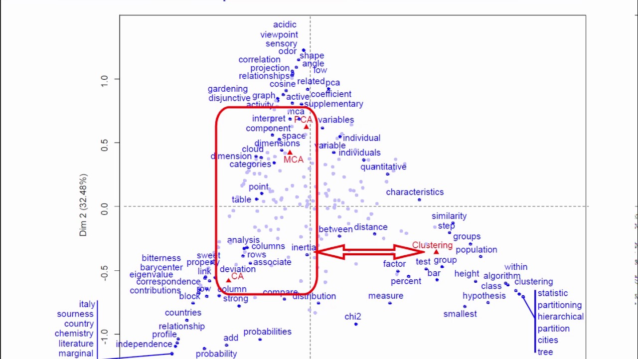
The video demonstrates how correspondence analysis (CA) can be applied to a small corpus of text descriptions for four data‑analysis methods (PCA, CA, MCA, clustering). After collecting the textual descriptions, a word‑frequency table (1,852 unique words) is built, then reduced to 246 words by keeping only those occurring at least ten times. The presenter explains preprocessing options (stop‑word removal, stemming, grouping) and highlights the property of distributional equivalence, which justifies aggregating words with identical profiles. Statistical foundations are covered: chi‑square test, phi‑square (0.792), inertia, eigenvalues (0.35, 0.26) and the proportion of inertia explained (77% by the first two axes). A simultaneous CA plot is interpreted: the first axis separates clustering from the factorial methods; the second axis distinguishes PCA (top) from CA (bottom) while MCA lies near the centre. Specific word contributions to each axis are discussed (e.g., “clustering”, “hierarchical” for clustering; “correlation”, “projection” for PCA; “probability”, “marginal” for CA). The stability of the results under different word‑count cut‑offs (5 vs 10) is shown, confirming robustness. A brief historical note mentions Jean‑Paul Benzécri and early CA applications to literary texts. The tutorial concludes that CA provides a clear, interpretable visualization of word usage patterns across the methods.
Chapters
In this video, we are going to see an application of correspondence analysis to a specific subject: text data analysis. The aim of the video is to illustrate the correspondence analysis course with a real example showing how correspondence analysis can be used to analyze a corpus of text data. More precisely, the data we are going to work with are the text descriptions of the 4 data analysis methods of this course. Principal component analysis, correspondence analysis, multiple correspondence analysis, and clustering. We have gone and got these texts and then built what is known as a word frequency table. Each column represents a data analysis method and each row a word that has been used. The entry in the ICE row and J's column counts the number of times the ICE word has been used to describe the chase method. In total, we have 1,852 different words that have been used. Specific data preprocessing methods for text data analysis can either be used or not before moving to correspondence analysis. We recommend doing preprocessing when the corpus of text is not too large. Words like, for example, then, therefore, and, etc. Have been removed from the analysis so as not to overload the graphs. But anyway, leaving them in wouldn't change the results much. Also, it's possible to group together words with the same root, like reduced, reduction, reduces, for example, as well as singular and plural versions of the same word. We haven't done this here. What we have done is kept words used at least 10 times and put the rest aside. Let's remind ourselves of one quite remarkable property of correspondence analysis: distributional equivalence. This is an extremely useful property when analyzing word frequency tables. What it means is that if several words have the same profile, we can group them together like a single entry before doing the analysis, by adding their word count totals. The correspondence analysis of this simplified table will give exactly the same results as a correspondence analysis on the original table. This immediately calms the debate about whether we should group together words with similar meanings, singulars and plurals, etc. Thanks to distributional equivalence, we know that if these words have the same profile, it doesn't matter or not whether we group them together. The results will be the same. Our final word frequency table has 246 words. Our goal is to analyze this table of word frequencies. Our first idea, which is quite simple, is to look for words with high frequency. For example, the word variables has been used 132 times to describe PCA. We might want to conclude that PCA is therefore a method that is particularly related to the use of variables. But before saying that, we quickly realize that the word variables is also the most used word overall: 294 times. So, really, there is nothing particularly interesting about this word, and its use 132 times for PCA is not so surprising. Clearly, we should really be looking at the marginals of the table. This is one of the most important things to do in correspondence analysis. What is our goal? Well, it's to visualize a word frequency table using correspondence analysis. Before getting into it, here are a few historical nuggets. The first applications of correspondence analysis, at the start of the 1960s, were actually for analyzing text data. The person was Jean-Paul Benzécri, who created correspondence analysis, and he was quickly followed by the whole French data analysis community. Jean-Paul Benzécri's first PhD student was Brigitte Escoffier, who defended her thesis in 1965. In her thesis, there are lots of very important theoretical results for correspondence analysis, including the transition formulas and reconstitution formulas. Their methods were applied to text data. One of the first studies was on the play Phèdre by Racine in which the characters of the play were contrasted with the number of times they each used certain words. This was one of the first text frequency tables analyzed by correspondence analysis. There were also tables looking at associations between verbs and nouns, the number of times each verb was associated with each noun, and tables looking at rhymes, the number of times various words were rhymed with other words, etc. All of this, text data analysis. Before beginning to interpret the plots, let's look at the inertia and percentages of inertia. The chi-square statistic, and the extremely small p-value associated with it, indicates that there is an association between word use and method. We can also calculate an indicator for associations between the 2 variables, that is the phi-square. Here, it's 0.792, and at most, it could have been 3, because 3 corresponds to the maximum number of non-zero eigenvalues. 3 is the minimum of the number of rows minus 1 and the number of columns minus 1. So the value 0.792 is relatively high, which means that there are some strong associations between words and methods. This means that certain words are indeed used predominantly to explain certain methods over others. The first 2 eigenvalues are quite large. 0.35 and 0.26, which means that an interpretation we do of these 2 axes will be based on a lot of information. Remember that, at most, an eigenvalue can be equal to 1. Looking at the percentages of inertia, we are able to say that the first 2 axes represent 77% of the deviation from independence. It's entirely reasonable to consider that this is a high number and therefore simply base our interpretation of results on these 2 axes. So here is the simultaneous representation plot for our example after running correspondence analysis. We can see the rows represented, the words, in blue, and the columns, the methods, in red. In order to make the plot easier to interpret, We could put labels only on words that most contributed to the construction of this axis. Straight away, we can see that the first axis separates clustering from the factorial analysis methods. This separation is very clear and shows that classification is described using specific vocabulary. Which words are overused to describe clustering? No surprises here. Words like clustering and hierarchical, of course, but also words describing the method, like partition, tree, within, clustering, class, etc. In contrast to this, to the left, we see words used more often to describe the factorial analysis methods. However, these words are spread out all along the 2nd axis, which contrasts PCA at the top with CA at the bottom. As for MCA, its coordinate value for the 2nd axis is close to 0, which means that it's a method that uses, more or less equally, the vocabulary coming from PCA and CA. This is why its coordinate value is in the middle. The terms at the top left are overused to describe PCA. These include words used in the examples, like sensory and odor, but also words like correlation, angle, relationship, projection. Bottom left, we have words used more specifically to describe CA, like probability, marginal, independence, barycentric, as well as words connected to the Nobel Prizes example, words like prize, Italy, chemistry, etc. The term chi-square, bottom center, is itself frequently and equally used for both CA and clustering, but rarely for PCA and MCA. Going back to the data table, we can confirm this: the word chi-square is used 10 times in CA and 11 times in clustering, but never in PCA and MCA. This slide summarizes the main interpretations that we have just made using the simultaneous plot. The inertia of the first axis is 0.35, which is high. This means that the first axis clearly separates clustering from the other methods and that the words used to describe clustering and those used for the other methods are quite distinct. If the first eigenvalue had been equal to 1, this would have meant that the words used to explain clustering had been exclusively used for that, and that no other words force clustering. As the eigenvalue is not really close to 1, this means that certain words have been shared across the different methods. However, as the eigenvalue is still relatively large, it does indicate that there is a specific set of words used overwhelmingly to explain clustering and not the other methods. Similarly, the second eigenvalue is also relatively large, which indicates that the vocabulary used for PCA has some clear differences to that used for MCA. One last question to ask yourself when deciding the analyzed text data: what is the minimum word count starting from which you choose to include words? In our example, we kept words that were used at least 10 times. But what happens if we choose 5 or 20 instead? Well, we have done the analysis again using a cutoff of 5 words, and we can see that the results here are quite stable. The positions of the methods are quite similar to before. As for the words, certain ones that were used between 5 and 9 times have strongly contributed to the axes and can therefore be found on this new plot. As for the words used at least 10 times, Their positions haven't changed much. In conclusion, our interpretation of the positions of the methods and the positions of the words will be very similar to before. That's all for this application showing how correspondence analysis can be used to analyze a corpus of text data.