Introduction to Quantum Computing in Wolfram Language

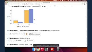
So the environment that you see, you know, is a Wolfram notebook. So in this notebook you can type text, you can have like, you know, your coding, Wolfram language, you can have, you know, visualization. Literally you can have everything. So it's an integrated environment. So first thing is that like, you know, as you may know, like, you know, Wolfram Mathematica, it has more than, you know, 6,000 building, you know, functionalities. Each of those functionalities, they are for a specific core area. I don't know, calculus, you know, algebra, like, you know, machine learning. And then like, you know, very recently, since last year, like, you know, we have been working on like, you know, developing a collection of functions for doing any sort of quantum computation in a finite dimensional space. So one more time, like, you know, it's any quantum computation in a finite dimensional, you know, Hilbert space. And what we call it is basically is a packlet. So packlet is basically like a collection of functionalities that are interconnected. And after installing the packlet, you can have access to all of those functions. So first step, you just need to evaluate this code to get what we call as Wolfram quantum framework. And as of now, these are the list of functionalities that we have supporting any quantum computation. The beauty of like, you know, having packlet is that like, you know, then very similar to any other function that you have involved in mathematical. Like, you know, you see here, like, you know, if you click, you know, on that, you would see like, you know, the documentation page. So each of, like, you know, these functionalities, they have their own documentation page. And like any other documentation, like, you know, the format is the same, like, you know, basic examples, properties and like, you know, can find, you know, other, you know, for example, I don't know, this is the list of, you know, functions that we have. You see like, you know, basis objects, you know, manipulation of that entanglement circuit so that, that, that's the collection that we have. So like, you know, after installing the packlet, like, you know, it's like you have those, you know, 20 something like, you know, quantum functionalities with the corresponding documentation. We did our best to have a documentation with no issue, but they might be some minor issues. If you spotted anything, please let us know and we would correct that. The main purpose of this session is having an introduction to quantum computing using our framework. So I'm going to start with something very basic at the very fundamental level. The way that we deal with any, any quantum computation is like this within some process, whatever that process, like we are going to Discuss about that very soon. But, you know, within a process, what we do is, you know, at the very end we prepare a quantum state. And that quantum state is stored like, you know, in one or many physical systems. In quantum theory, the simplest system that we have is a system of, you know, dimension two. Basically that's a system that like, you know, in the simplest case, you can describe it by a vector of two with two amplitudes. And those amplitudes, they can get like, you know, complex numbers. They can be pure, they can be complex. But what you see here, like, you know, let's say that you know, something happened and at the end, like, you know, you prepare like, you know, this quantum mistake, okay, quantum state. Like, you know, after evaluating that like, you know, quantum state in a framework like, you know, is an object and this is basically the summary box for that object. Don't be scared of the summary box. If you want, you can look at the traditional form on Mac. The short key is command shift T. So that's basically the broadcast notation, the traditional form. I'm using the short key or you can simply wrap it around traditional form and you can see it. That short key was literally applying this function on that state. The beauty of like, you know, these objects is that, you know, they contain lots of interesting information that it can help you to get like, you know, to have an idea like, you know, what you're doing. Like, you know, what is a picture, what is this state? It's a purest state, form of nine. Entropy is, you know, zero. It's one physical system. The number of quimension, etc. Etc. But anyhow, like, you know, let's focus on the, on the big picture. So physical process happen. Like, you know, we prepare a quantum state and then the next step that we do is we do measurement. Remember like, you know, in quantum theory, measurement is very different from any other transformations or like, you know, whatever transformation, whatever process that is happening on quantum system measurement is different. So what I'm doing here and think about it like, you know, very similar to like other functionalities that we have in both a Mathematica, a function, it acts on another function and then. And the results is an outcome. So here like, you know, our quantum measurement acts on basically this is the input for this function. I'm saying that like, you know, measure it in, you know, computational basis. There are some details like, you know, for example, if you do not know, like, you know, how to do that, like just, just look at the documentation. So this is the documentation and like, you know, it's kind of contains all the information that you need regarding that function. But anyhow, let's again let, you know, let me just briefly review and then I'm going to go into the detail. So a state is prepared and then at the end you do a measurement. In our framework, because like, you know, we have all other functionalities involved from Mathematica, you can calculate the corresponding probabilities. Remember, quantum theory, the best description at the end is giving you with what probability you can get the corresponding outcome. And this is what we get out of, like, you know, this spatial state. Okay? So like, you know, that's basically the bar chart of like, you know, that measurement. That's not what is happening in practice because these probabilities, like, you know, Wolfram Mathematica, it calculates them exactly, meaning, because, you know, we have, you know, statistics, probability functionality. These are the exact numbers in reality, like, you know, in experiment. Just let me show you, like, you know, a spatial case that I have simulated an experiment. You have to basically repeat the ex. The measurement and you would get a collection of results. Okay, so in this very spatial case, you know, what I'm doing here, I'm simulating the measurement results and I'm saying that do it 20 times and this is basically what I'm getting here. And then out of that, you can calculate the corresponding frequencies. So what I'm doing here is I'm just. Let me just show you these steps. I'm just telling like, okay, count them. There is always an association. It says like, you know, for one, you know, you got 18 results. For zero, you got two results. And then the next step, I'm just saying I'm going to normalize that based on like, you know, let me just use, you know, this syntax which means, like, you know, check this, you know, outcome here. I'm just saying that, you know, normalize by total, you know, because I want to get, you know, the probability. It's just like, you know, how to get the probability. This is basically, you know, the frequency that we get. This is. This is what happens in experiments, of course. Like, no, in reality there are noise and many other, you know, complexities. But anyhow, like, you know, that's what you would get. And you can, like, you know, compare them together, you know, easily. But the, the orange one is like, you know, the exact, like, you know, that's exact calculation. And the blue one is what you get out of the experiment. Please note that like, you know, because again, you know, in Wolfram language, we can have, you know, Symbolic calculation. And again, you know, all of those statistics and probability functionalities, the results that we calculate, I know, like, you know, I refer to them as a sort of, like, you know, simulation, but they are exact. That's why, like, you know, on purpose, I put it, like, you know, as exact. And this is a very unique feature about our framework. Like, you know, if you want to reproduce, like, another measurement results in other, you know, quantum frameworks, the best they would do is they run it, you know, a couple of times, I don't know, 10, 24 times, and they just tell you, like, you know, what counts for each measurement. This is the core idea of, like, you know, any quantum computing. That's it, okay? Like, you know, it's prepare a very particular state and do a measurement. And for the measurements, you know, at the experimental level, we get, like, you know, collection of results. And then based on that, you know, we want to do a very particular, you know, computation that. That's it. The biggest headache is usually like, you know, how to prepare a very particular state that is suitable for a very particular goal, for a very particular, like, you know, objective that we have and how to prepare that. Okay, so that. That's the whole idea of, like, you know, developing a quantum algorithm for a very particular purpose. Okay, but let me just comment a little bit more about, like, you know, quantum measurement because, you know, remember that, you know, in quantum theory, you can do quantum measurement in many possible ways. For example, the previous example that I showed you was, let's say, like, you know, pretending that this is a simulation of an actual, like, you know, quantum processing unit. It was in computational basis 0 and 1. You can change that basis. You can do it, for example, in Pauli X and you would get, you know, the corresponding probability. So these are the results in Pauli X. And this is the result like, you know, in for, like, you know, computational basis. So that for that measurement, you have lots of freedom. Okay? So that's the big picture. A quantum state, you would do a measurement. And for a measurement, like, you know, the best is like, you know, you can calculate some, you know, frequencies. And then you have to ask, okay, what I can learn out of those frequencies? Okay, what kind of, you know, operation I can do with that? So first, what. What quantum state given, like, you know, any initial state, like, you know, let's say that, you know, you. You prepare your system in a particular state and then you want to transform that estate. In quantum theory, this transformation can be done in many different ways. Okay, for example, like, you know, One possible way is doing it in a unitary way. This is what we usually have as quantum operator in quantum theory. So what I'm doing here, I'm just saying that, you know, okay, prepare a very particular state and then apply like, you know, Pauli x poly X in two dimension is, you know, it's literally the same like, you know, not operator. And of course, I'm sure you guys know that like, you know, you go from zero to one. So this is the transformation. Like, you know, I'm showing you the simplest case but like, you know, then the next step for any quantum algorithm is what is the collection of, you know, transformation for a very particular objective. What, what we can do, like, you know, how we can compose a very particular, you know, transformation. So let me focus on like, you know, the idea of like, you know, transformation, like, you know, how I can change the state. Just like, you know, a common terminology that we have in quantum theory because again, like, you know, the most popular, you know, quantum systems, quantum system in two dimension, like, you know, spin half system, for example. Like, you know, let me show you like, you know, a case that I'm preparing, like, you know, a random pure state. And I'm just looking at the amplitudes. Okay? So this is literally like, you know, for this basis, you know, this is the amplitude and that's the other one. This is basically the same like, for example, in our framework, the another term that we have for that is a state vector. But you see, like, you know, behind the scene, you know, for us, a state vector is a sparse array. And if you want to see like, you know, the actual form, just like, you know, look at the normal. Okay, so that, that's what you get. Of course, you know, when you're looking at this state, you know, vector, remember, like, you know, the order like, you know, this amplitude correspond to what, you know, element of your basis either, you know, if you don't know that, for example, look at the amplitude because, you know, it shows you like, you know, the keys here are basically like, you know, the element of the quantum basis that you are using. But anyhow, like, you know, so for the simplest quantum system, you know, we can describe it by vector, a vector of two elements that can be like, you know, complex. Another way of, you know, representing that is by a vector in three dimension. And this is what we usually call as a block vector. Each of these objects, each of these objects that we have in our framework, they have a long list of properties that you can find in our documentation page. Oops. I Went to the documentation for. Let me just show you the documentation page here. And if you click on the details, there is an explanation here. For example, here, block spherical coordinates, coordinates of the quad, block cartesian. Like, you know, so it gives you the cartesian coordinates. So this is basically the cartesian coordinate. And this is, you know, the spherical coordinate of, you know, r, theta and phi. And this is basically the three dimensional, you know, visualization. So you have a sphere and like, you know, this vector represents the same state as what we have here. This representation is very popular. Like, you know, those of you, if you want to work like, you know, in this field, you need to know more about like, you know, block sphere. Because this is one of those knowledge, like many times when you want to describe anything, we refer to the, you know, block vector and what happens to that? Okay, now let me consider, let us focus on a very simple case. Okay, so what I'm doing here is that like, you know, I'm preparing like, you know, a quantum state in a zero state. I guess you already noticed, like, you know, I haven't mentioned that. But look at here. Like, you know, the quantum state is taking a string as an input. So this is exactly the same as doing it as a vector when the first element is 1, sorry, and the second element is 0. So this is by definition, that's how we define like, you know, zero state. And as you notice, like, you know, all other functionalities that you have in Wolfram language, like, you know, you can apply it on the, on the top of, you know, quantum objects. But anyhow, let us continue like, you know, with our story. So what I'm doing here, I'm just doing, you know, a simple transformation. I'm saying that like, you know, this function, which is a rotation with a given, you know, vector is acting on that initial state. And that initial state is basically your zero state. And then I'm looking at the block plot of that state. We can just, you know, wrap it by manipulator. And you see here like, you know, it is clear, like, you know, it's the rotation around the y axis that we have here by corresponding angle theta. Okay, so it's just a simple transformation. Now let me make a composition of these operations in two steps. I'm going to say first step, I'm going to apply rotation. And you see here, the notation that I'm using here is a functional notation. Here I'm just using the prefix notation. Okay? It's just like no different syntaxes that we have involved from language, but Anyhow, what I'm doing here, I'm just saying that, you know, first apply rotation around Y by the corresponding angle theta on this initial state. And on the result, apply rotation around C. And as you can see, like, you know, for example, you know, this is the rotation around Y axis. And now a rotation around, you know, z axis, we can go from a final state, we can go from an initial state to a final state. So the idea of like, you know, a composition, like, you know, this is what we usually call as a composition, like you know, two transformation apply on a particular state. This is basically the very fundamental idea of like, you know, a circuit. So whenever we talk about a circuit, a circuit is literally like, you know, a collection of like, you know, different operations. And those operations, like, you know, I'm on purpose, I'm saying operation in the most generic term because they can be even non unitary, non trace preserved. They can be anything. It can be a noise, it can be, you know, stochastic. It can be a quantum channel. It can be literally anything. But here, you know, I'm just considering the, the. A very simple case, like exactly the previous situation that first rotation around Y, then rotation around C. Now this is basically in language of circuits. The, the most common thing about the quantum circuit is, you know, the corresponding visualization which is what you see here. Each vertical wire, each horizontal wire, it represents a quantum state. And each of these boxes is basically your transformation. And here we should read from left to right. Okay? So it means this guy here, you know, rotation around Y. It acts first and after that the Z. So remember like, you know, I'm writing it here, like, you know, left to right and that that's the very first operation that is happening. There are some like, you know, the way that you can build your circuit. I'm gonna show you, you know, some complicated examples. But anyhow, like, you know, either you can literally the way that I'm doing it here, include your objects. But you see here like, you know, somebody would say, ah, look now this is redundant. I'm just repeating, you know, quantum operator. Can I get rid of that? Oh, yeah, of course, you know, we can do that. You know, we also support like, you know, those shorthand notations. So basically, literally like, you know, whenever you have quantum operator wrapped around that, you know, you can just remove that and that, that maybe helps with writing the code or reading that. So it's like, you know, basically rotation around Y by the corresponding, you know, angle. Rotation around Z by the corresponding angle. And you can easily again, like you know, check that, you know, they are the same. These two are the same thing. One very important feature of LOCK in a Wolfram language is that you can do symbolic computation. As you can see here, you know, this circuit is a symbolic circuit. I'm not assigning any value to parameter, you know, theta and phi. Okay? They are literally like a symbol. And you can. What you can do is you can say, okay, this circuit. Now I want it to act on an initial state. So the way that you can do it is just like, act it. Like, you know, that circuit. I call it, you know, comp. And, you know, it can act on any quantum state, whatever is that quantum state. Okay? For example, this. This is a state representing in a 1 qubit. So it can go even with a random Q or like, you know, whatever state you like. Many times we prepare all of our queued bits in the ground state, meaning all of them are in the zero state. Because that's the most common way of dealing with quantum systems and quantum computing. One shorthand notation is just don't give any input. Whenever you are not giving any input behind the scene, what we do is we are going to set whatever quantum system that you have, all of them at the ground state zero. Basically, this operation that you see here, quantum state zero. And then like, you know, this circuit acting on that is the same as this operation. But anyhow, like, you know, this is a transformation, like, you know, a transformation of the state. And then you can look at, like, you know, the amplitude. And these are the amplitudes that, that we got. As you can see here, these amplitudes are still, you know, in the symbolic form. Okay? Like, you know, this is one important thing that to remember about, like, you know, go for language. It has a very, you know, strong feature. Maybe the characteristic trait of like, in a Wolfram language is that you can do symbolic calculation. Okay, now, so let's. Let's jump. Like, let me give you more information about, like, you know, okay, this composition of operation, which is basically the wrapper around them is our quantum circuit operator. You can do whatever you want. Let's try to read it like. So here I'm just saying that, you know, poly X, poly Y, and then rotation around X by the angle theta. This is basically the collection of like, you know, gates that we have, like, you know, like, that's how we would call them, you know, in quantum computing. And all of them are acting on the same wire on the same quantum system. Very interesting feature that we have in our framework is called order. So you can Say, you can specify a very specific order. You can say, look, I want, you know, this rotation to act on the second quantum system, okay? So that's how you would do it. You would just, you know, specify a rule. And this one would say, okay, this rotation goes to the second system. And if you look at, like, you know, again, like, you know, what I'm doing here, I'm just using the shortcut for traditional form, like, you know, on Mac is command shift T. And as you can see here, like, you know, so X is on the first. After that, Y on the first qubit. And then, like, you know, you have rotation on the second one. Remember, like, you know, unless these commute, like, you know, the order that you are writing them. Like, you know, is very important. So that's the rule of thumb. Like, you know, those of you who are new to this field, remember, like, you know, the order that you're writing. All those operations are very important. Or another example, like, you know, look at, you know, this example, what I'm doing here. I'm just saying that, you know, okay, you know, this time, like, you know, I would like, you know, poly Y to act on the third qubit. So this time we are going to have, you know, three wires. For the first one we have like, you know, poly X, second one rotation around X, and the last one is Y. So that's how, like, you know, we can, you know, build, you know, a composition of different, you know, gates, different, you know, transformation for our quantum systems. Of course, the examples that I have shown you so far, like, you know, all these examples as you. As you see, like, you know, each of these transformations, they are acting on a single qubit. You can have, you know, more complicated cases. Like, you know, for example, like, you know, this is a fancy control gate which is acting simultaneously on four quantum systems at the same time. Basically, you cannot decompose it into a, you know, chronicle product of like, you know, four different operations. Okay? It's acting on that whole, you know, space at the same time. Okay? So your gates, your transformation, they can act on a single. They can act on many of them, two or more at the same time. And again, like, you know, look what I'm doing here, I'm just going with the control. And then I'm saying that, you know, the operation is X, this is control one. So I'm just saying that, like, you know, number one and number two, if they are one, act it. And then this is basically control zero. So, like, you know, these are like, you know, the arguments for our control gate. And again like, you know, if you don't know how to use like, you know, these functionalities, just, just look at our documentation. It has many examples and each of these named, you know, operations like, you know, they are explained here in detail. Whenever you are looking into the documentation, especially for circuit operator, please remember that many of the things that you see here, they are actually quantum operators. So if you go here, let me show it one more time. And under the details, you didn't see any description of the control operation. It means it is under the documentation for quantum operators. Let me just go at the very documentation. So if we click on quantum operator and here like you know, you would see it like, you know, all this, you know, all of them are collection of, you know, control gates that we have here. So we can find like the detail here. Okay, so that's the one that I was using. And each of like, you know, these operations, they have a full name or they have a short name. Like, you know, you can use either one. Now let me just give you like a very specific example regarding like, you know, what we usually call as a quantum algorithm for a very particular, you know, go. And I'm gonna use, you know, a textbook example which is, you know, Grover quantum search algorithm. Okay, so the idea is like this, let's say that like now we have this Boolean function which is simple like you know, the, the like you know, and, and then not on the second one using like, you know, the other building functionalities involved from Mathematica. You can easily find like, you know, what are the solutions of this Boolean function? It's a trivial case. It is clear that if Q1 is true, Q2 is false, like you know, you will get like that, that's a solution. You will get a true value for F. Okay, now let's, let's what is the quantum process for finding, you know, this solution? Okay, so that quantum process is going to be like this. You would start by preparing your physical states in the ground state. You would apply some transformations and then you would do a measurement. Remember all of those transformation. At the end of the day they prepare a very particular quantum state. So any quantum algorithm is like a very specific quantum state followed by the measurement. Remember like, you know, measurement. That's the only way that we can extract information out of like in our quantum system for this very particular case. Like, you know, I guess you already noticed when I was showing you the documentation for quantum circuit operator we have a long list of name operators named circuits. So these are very common circuits that we have for a very particular algorithm. And let me focus on again. As I told you, that's a textbook example Grover search. I look at like, maybe it's better if I just show it to you that like, you know, we have all the completions. So when you just type it like, you know, it shows you, you know, complete list of like, you know, named operators that named circuits that we have. I don't know, like, let's just look at the magic one for preparing like, you know, bail estate. And that, that, that's what we have here, by the way. Like, you know, all these features, like you know, this gray box, like you know, that particular composition that you may not like it to see it on the top. Like, you know, all of them, like, you know, you can easily customize them using are labeled functionalities. And let me just find it for second diagram. It's here, you see, like, you know, what I did was, you know, just, I just searched through the documentation and that's the diagram for, you know, quantum framework. And these are all the details, all the options that we have for circuit visualization. I know like, you know, many of our users are using, you know, Wolfram language for visualizations. So like, you know, we have lots of options. You can do a lot. But, but anyhow, let's, let's, let's move on. So the input, the argument here is basically that Boolean function. I'm just saying that, you know, look, you know, I'm looking for Grover search algorithm. This is a Boolean function. And this is a circuit diagram that we have the first, you know, step like, you know, the one like, you know, is inside the gray box. You know, for Grover search algorithm, it is usually called. Diffusion step. Oh my God, for a second I forgot the terminology. And the second piece that you see here is amplification. So what's, what's happening here, like you know, is practice. And by the way, like each of them, let's say that, you know, you are interested in just looking at the global diffusion and. Did I block it? Yes. So I'm, you know, this will be functional very soon. Let me just make it local note of the that I'll fix it very soon. But anyhow, like, you know, each of these pieces. Let me also check if we have go. See is it the same case for phase? Definitely fusion. Oh, Okay. I have broken that. So I'll, I'll fix it in a sec. Each of these pieces basically like you can extract it. You see, like, you know, the named Operators, they were there. But let's continue. So what's happening here is that, you know, during the first step, the. The gray box, we are saving the information about the solution in an ancillary qubit. And then in the second step, we amplify the. Basically the amplitude of that. That very particular solution. Okay, The Grover search algorithm, like, you know, remember login, it has two features. This is the one which is based on, you know, Boolean oracle. There is another one which is basically Rover. Show it separately. Without using the ancillary qubit. Okay, so there are. Whenever we, you know, when you are looking into the literature, there are two borrower search algorithms. One of them is ancillary qubit. With the other one without that. In one case, we are saving the solution in ancillary qubit. In the other case, we are saving the solution in the overall amplitude. Like, basically, we are adding a negative phase in front of like, you know, our. Our superposition. Make sure, like, you know, you understand the difference between the two. But anyhow, let me just focus on, you know, what's. What's happening here. So first, you know, I need to prepare my quantum state. So, and this is, you know, basically the step for preparation. So what I'm doing here, I'll make sure that, like, you know, the ancillary qubit is prepared in state one. That's why, like, you know, I added a not state here. And then, like, you know, I add Hadamard, you know, on all of them to have a sort of like, you know, you know, uniform superposition. And again, you know, let's read like, you know, the code here. And this is again, you know, one of the other things that by design, you know, we spend so much resources making sure that, you know, the code is also readable, not applied on the third one. And then we have Hadamard, a collection of Hadamard on three qubits. There is like. Instead of like, you know, this design, you can go like, somebody would say, like, you know, look, you know, I want to do it like this. I want to say like, you know, how the mart is acting whoops. And 1 and 2 and 3. So that's. That's the same thing. Okay, again, like, you know, this particular design, like, you know, it's maybe easier than this one. But anyhow, like, you know, you can use, you know, either one, the second one, like, you know, it's good because sometimes you may want to act. I don't know how to mod only on some specific, you know, qubits without and skipping some of them. Okay? So that's why, like, you know, giving it as an order, maybe it's better than just giving it, you know, in this form. But anyhow, like, you know, that's our preparation. And now look. Look what I'm doing here. So here, it's basically like, you know, I'm. I'm making a composition of some circuits. Remember, this is one circuit. This is another circuit. And look how it is done. I'm saying that, like, you know, the notation that we have here is just for droid composition. I'm just saying that, okay, start with, like, you know, the circuit that I call prepare and then grover and then measure qubit number one, qubit number two. And this is a circuit that I have constructed out of that. So get along, you know, remember, like, you know, this is another way of, like, you know, thinking about, like, the composition. It's literally like, you know, whatever operation you have as far as, like, you know, it is an operation. Remember, operation means transforming the quantum state. You can have, you know, their quantum. You can have the, like, you know, their composition. The first one is a quantum circuit. This is a quantum circuit. This is a ground measurement operator. But you can, you know, compose them together. Okay, so this is our circuit. And now I'm saying that, you know, okay, this circuit is acting on, you know, a ground state of qubit number one through qubit number three. You can say explicitly like this. You can say that, you know, we have three estates. All of them are preparing quantum state zero. That's one way of, like, you know, doing that. Or again, like, you know, as far as you are dealing with the register state, this is sometimes what we call as a register state. And by the way, this is another way of, you know, doing exactly the same. So you can, say, go with the register state of three qubits. Okay? So this is the same as what we have here. The same as what we have here. Many times, like, you know, if you see me or, you know, other people that go from doing. Do coding, you know, in our framework, you go. We go with the shorthand representation. But anyhow, do whatever way that you are more comfortable. And because we had, like, you know, the measurements, okay, so the result, you know, is an object which is quantum measurement. Okay, because again, like, you know, we had, you know, measurement operator here. You see here, like, you know, that the double, you know, horizontal line on the top, that's basically a classical wire. You know, that's the wire that you're saving, you know, classical information. And by the way, you know, one more time, all the labelings that you see here, the label on the left, the label on the right, whatever you want, like you're showing, like, you know, the classical wire or not showing the classical wire, you can customize them whatever way you want, you can eliminate it, you can change the color, you can make it brighter, you can make it darker. Like you know, you can, you can do whatever you want. But again, let's see, like, you know, I did, you know, all this operation and I did like a measurement. Now, now the question is, okay, so what now let's, let's look at the probability distribution. So what I'm saying here is just return the probability plot of the results. And remember, because we were measuring 2 qubits HQ bit 2 possible outcomes. So the potential outcomes are 4. Of course, I'm kind of cheating. I'm using a simple example that shows you directly the result algorithm is usually more complicated than that. But anyhow, look at the outcome with the largest probability. Here is a very spatial case, you know, with probability 1, you'll get the case that Q1 is in 1, Q2 is in 0. Now let me remind you, what was the solution? The solution was the first one true, the second one false, 1 and 0. And that's exactly the solution thing. Okay, so that's basically like, you know, a very simple, you know, quantum algorithm for a very specific, you know, objective. And of course like, you know, there is a hot topic for any quantum algorithm is like, you know, how much it is, you know, better than, you know, classical counterparts. Okay, so that, that's a completely different topic. Like, you know, to be honest with you, you know, I'm not an expert on that but like, you know, I understand it, but I would leave it to especially like, you know, mathematician or you know, computer scientists with quantum expertise. Like, you know, they can elaborate more on that. There are lots of, you know, textbook on that. Let me just mention one other thing. Like, you know, you notice, you know, the way that I created my overall circuit was using this fancy notation and right Composition. Etc, etc. Okay, so you may have a different mindset. You may have, you know, look what I'm doing here. At the end of the day, it is also like, you know, a composition of bunch of circuits and the circuit number one is prepared, the circuit number two is over, and then I do measurements. So why not giving them as a list inside the circuit operator? Yes, that's, you can do that, you know, and you would get this result. The only difference is like, you Know, in terms of, you know, visualization. Because like, you know, now you're feeding each one of them as a circuit. We just wrap it around like, you know, that gray box and the label on the top. Like, you know, it's basically the composition of like, you know, whatever you do. But again, like, you know, if you don't want to see these boxes or if you don't want to see those labels, you can easily eliminate them. Okay. Like you can customize all of them. And of course, like, you know, this, you know, the result, it's going to be exactly the same as the previous one. Okay? So they're different only in terms of like, you know, visualization. That was basically a very, you know, simple introduction to, you know, quantum computation using our framework. So the way that I want you guys to like, you know, those of you who are new to this field is just think about like, you know, target state and then a very particular way of, you know, preparing that estate. Keep that in mind. At the very end you are always dealing with the measurement results. Okay? So it's a probabilistic like, you know, reasoning, if you want to think about it, like that's how, that's how we do it in quantum theory. And by the way, this is not the only paradigm to do quantum computing. The paradigm that I'm like, you know, explaining here is what we usually call as a gate based paradigm and majority of like, you know, quantum processing unit. The actual quantum hardwares out there, they know, they are claiming that like, you know, if we can trust them, that they are quantum. But anyhow it's gate based. There are some companies that are offering like, you know, a different approach. Like for example, like you know, like, you know, D wave, like for them is not a gate based, like, you know, approach to do quantum computing. In those cases, like, you know, for a very particular objective, you know, you would design like, you know, a Hamiltonian and then like, you know, that Hamiltonian, that very particular Hamiltonian would do the job for you. So it's a very completely different approach compared to like, you know, what, what we have here in terms of like, you know, experimental. Which one is better? Which one is like, you know, I, I don't know that that's a question for the experiment mentalist. And, and we should wait and see like, you know, monitor the progress in, in experimental advancement of like, you know, quantum processing units. So that was basically like, you know, what I had prepared for today. So if. There is anything that has not been one more time, remember like, you know, you just need to install the packlet after like, you know, installing the packet. If you do not, you know, quit your kernel, like, you know, the functions will be there. But if you quit your kernel, like, you know, yeah, you have to basically install the packet every time that you're creating your kernel. And of course everything behind the scene is done. But yeah, it's classical. Like, you know, we are doing a quantum algorithm on a classical machine. Okay. It's you can, by the way, like, you know, we have, we have it in your documentation if you are interested. You can send your queries from a Wolfram notebook. You can send your queries to a quantum processing unit. You can use either IBM quantum processing units. You can use anything that is available on AWS and just wait, get your result and then do whatever processing you want to do with that.