Quantum Operators, Time Evolution and Quantum Measurement
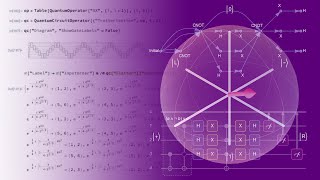
A walkthrough of quantum software tools for building and measuring quantum states. Learn to create Bell states, check entanglement with partial transpose, evolve systems in time using Trotter-Suzuki decomposition, and visualize everything on a Bloch sphere.
Chapters
Okay, hello everyone. Hope you're all doing well. Okay, let's start. Nick, you know, let's do some, you know, problem solving from quantum state, quantum basis. Like, you know, remember guys, like you know, learning any new topic, like, you know, it's always challenging. So like, you know, the more you challenge yourself, try to solve some problems, the better you would understand it. And of course, like, you know, this process, it's gonna be painful. By the way, like, you know, what you just saw on the right side of the screen is a palette. Like you know, under the palettes you can see like, you know, after installing like, you know, quantum packlet, you should be able to see that palette. It helps you like, you know, some of you asked like, you know, for how you can easily see the patterns for, you know, relevant definitions. As you can see, we added, you know, some, you know, we are planning to extend that. But like, you know, if you click on any of them, like you know how to do it, you know, create a quantum state. Like, you know, let's get one example. Like you see, this is zero state. Or like, you know, the measurement operator, second operator. So like, you know, and you can see the results. Okay. Another interesting bottom, like, you know, on that palette is reinstall the packlet. So, so it's basically, I know some of you, you had some issues, but like if you just click on that, you can basically reinstall the packet every time making sure that like, you know, you're using the very latest version. Okay.
It's equivalent to this command over here.
Yeah. Anyhow, let's go through our problem. So let's go with the first one. Let's see what we have. Create a random two dimensional pure state.
Should I do it?
Yeah, let's see. Like, you know, so it's clear, you know, it's a, you know, quantum state. And like, you know, this sound like, you know, Nick is going with the, like you know, the building names that we have. So it gives you a random pure state. Remember like, you know, whenever no dimension is given, automatically would assume you know it's happening in 2D. Another approach is just like, you know, what Nick is showing you here. Like you know, you can go with the generating your own vector. So what's happening the second time, second example is that like, you know, Nick is creating two random complex numbers and you can inject it as an amplitude. So the second option, like, you know, you may, like, you know, it may give you like, you know, some headache because it's not normal, as you can see. Nick is showing you the normalization factor, but the building it returns a normalized state both ways. You can create a pure state. The main benefit of using random pure is that you can easily generalize it in any dimension. You can easily go like 2, 3, increasing the number of states. Whatever you want to do. Okay, the next step. So let's say that you have your random. By the way, as we are discussing, feel free to type your questions and we would address them. So look at the examples. The first one is a random pure state in three dimension. The second one is a random pure state of 3D, the composite system. The first system has the dimension 2. The second system has the dimension 3. Okay, so like you know, random pure, like you know, helps you to easily create, you know, random pure state in any dimension. For any like you know, when we have a qubit two dimensional quantum system, you can directly visualize the block vector. So let's just visually create a random pure state in 2D and let's visualize. So it's block plot, you know, that's the property that you can ask. And that's basically your random pure state in block sphere. And of course like you know the, the vector, the red one, the block vector that you see there, you can either get the spherical coordinate of that vector or you can easily extract the cartesian coordinate. So for the one of them you have to ask like let's go the next one, spherical coordinate. So that's the spherical coordinate of that one. And likewise you can go with curtails and coordinates. Hey Nick, would you mind trying to go to 150 magnification? It is looking a little small.
Sure. Maybe even 200 all the way. It's too big.
Yeah, I think 150 is going to do it. Thank you very much. Okay, okay. Now like you know, one interesting, like you know the, the feature that you guys can do is, you know, I'm sure you already noticed but like you know, it's very useful going from one basis to another basis. Because whenever basis is not given, like all these cases, like you see, there is no second argument. So everything is done in the computational basis. Given a state in any basis, you can transform it in any other basis. For example, like you know, let's generate like you know, a pure random state in computational basis. Let's call it whatever we want to call it, state psi, whatever. Like you know, the notation is not important.
Just trying to organize it a bit better.
Random pure. Now like you know what's happening here. Like you know, this time like, you know, we specified that in that very like, you know, basis. So this time, like, for example, let's look at the formula. You see, this time like, you know, the formula is given in Pauli X. So like, you know, this is one interesting feature that you have. Like, you know, this basis transformation, it's a very nifty feature of our framework. So both for basically any quantum object, you can easily transform it from one basis to another basis. Just make sure that, you know, those basis is representing the same global space. So here, remember the first arguments that specifies what type of state and then the second argument tells you what basis here the basis is. Pauli X.
Can I just comment, because I was showing this yesterday and it's important to distinguish two different cases when you create a state in some basis like this one, when you provide an amplitude or name, right, it's going to just treat those amplitudes or whatever formal state you have in this particular basis. Or you would actually convert it from computational basis to this basis. This is like a different thing.
Yeah, so like the last example that Nick is showing, you are creating a state in computational basis and then you transform it into poly X basis. So it's basically a basis transformation. Remember like, you know, these two states are the same. Like, you know, it's just like, you know, in which basis you would like to see your state.
All right, okay.
So the next examples, like, you know, they are like, you know, trivial. Like, you know, we can just leave it to our users. It's just like, you know, creating a state and the transformation. Let's go with the composite one, which is a bell state. So remember that like, you know, those, you know, you can do that. Now let's go with the bell state. So now for the bell state, how we can do that? So like, you know, you see here we have a very particular superposition of, you know, five plus five minus. Now how we can create them, you can either go to bell basis and, and give an amplitude, for example, like you know, any amplitude. I don't know, let's go with symbolic amplitude A, B, C, D. Let's add the other two. So just show them all of them together. So you see, like, you know, this is the bell state and like, you know, each one corresponds to particular like, you know, bell state that we have. So when you want to create that particular superposition, you just need to specify the corresponding amplitude. So it's five plus. So we are going to put five plus one over square root of three and likewise for psi negative. So basically it's going to be D and A. So.
So it is 0, 0.
Yep. That one gonna be negative square root of 2. There's a negative sign. So that's the estate that we created. So that's one approach. Like, you know, in this approach, you know, what we did, we use a given name basis. Okay. Of course, another approach is literally creating that superposition using name state. Because we have a quantum state phi plus. So we can start by creating your quantum state 5 plus. Again, you know, this time we are using name states five plus. And then, you know, this is the definition of five plus. And then you can, you know, create a superposition. Now let's transform it into bell state. You know, that's the representation in bell state. And then what you can do, you can create psi minus. That, psi minus. And then for the superposition is literally adding them together with the corresponding coefficients that we have there. So there are different ways of creating quantum superposition. And these two states are exactly the same thing. So please keep that in mind whichever way you feel more comfortable. So just go with that. Sometimes, you know, people, they prefer like, you know, the amplitude. But when you are using the amplitude, you should know, like, you know, which amplitude corresponds to what basis. Or you can go with the, you know, summation of some quantum states. Okay. And like, you know, Nick already, you know, showed you, like, you know, the formulas and everything. So the second part of that question, which was about the formulas, you know, we already addressed that. Two over a square root of three. There's just a typo there that's showing.
Off a little bit of nice notation.
So, like, you know, what you see here, like, you know, the traditional form, remember, like, you know, on Mac is command shift T. Like, you know, it's just, you just need to evaluate that. And then, you know, command shift T. Like, you know, it shows you, like, you know, the corresponding formula. Okay, now let's like, you know, the next step. Like, you know, we are doing, you know, some simple, you know, operation that we can do our state. So we created that superposition this time. Like, you know, we want to trace out the second system. So the function to do that is, you know, quantum partial trace. So let's. So that's our, you know, state, you know, remember, like, you know, it's in two dimension. It's a composite system. So we just take quantum partial trace. So the first argument is the state. The second argument is the system that you want to do the partial tracing.
We can't do that because it's a four dimensional One.
Oh, then let's go with like, you know, transform it in the computational basis. Let's go to two by two. Oh yeah. So just like, you know, let's clarify like, you know, what, what happened there. So you can define your bell state in a big system of four dimension and say that, you know, look, this is my system. Like, you know, it's four dimension. So physically it means you have only one single quantum system. Or you can break it into two subsystems. You can say that, you know, look, look, look, you know, what is happening in reality is like, you know, it is two cubits together. It's a composite system. But like, you know, in our framework, you know, we understand them like, you know, and then the next step, like, you know, after partial tracing, of course we know that, you know, it's a mixed state. But like, you know, we are just checking that, you know, whenever we do the partial tracing on the top of pure state, we are going to get a mixed state. Now what we can do, for example, let's call that after partial tracing, whatever is that state. Let's call it, I don't know, let's call it R, for example. One interesting feature, remember, it's a mixed state, so we can purify our states. So purification is a very common process in quantum information. So the syntax is just purify that. So what's happening here is that we are using an ancillary quantum system. We go to a higher dimens and in this higher dimension, your state is basically pure. Now if you want to recover the original state, so if you want to recover that, you just need to do the partial tracing over the ancillary qubit. So let's just take the partial trace of the second one. You are going to recover your mixed state and you can easily test that that's exactly the same as the original mixtape R that we started with. Okay, so it's just like, you know, purification, like, you know, it's a very common process that like, you know, we have in quantum information. So just in order to purify a mixed state, you know, just add, you know, ask for the property, purify. Of course, like, you know, if your state is originally pure, if you purify that, you know, it's not going to change anything. So remember, purification is always means going into a higher dimension. Okay. Going into higher dimension. Okay.
We'Re still gonna go into high dimension. Just.
Yeah, it's. Those amplitudes are basically, it's a trivial process. Let's put it in this way. Yeah, I Don't know, like, you know, just quick comment. Remember, like, you know, when you purify, when you go to a higher dimension, the amplitudes, they are basically the square root of like, you know, the amplitudes that we have in the mixed state. Therefore, you know, there are some cases that, you know, people are interested to go into a higher dimension without changing the element of your density matrix. So one more time, like for example, Nick, let's, you know, create, I don't know, let's go with symbolic, you know, mix states. Like let's go ABCD and let's purify that. I know it's, you know, unknown because like, it's not clear it's mixed or not. And let's look at the formulas you see here. Like, you know, we are going into higher dimension. And then like, you know, the relationship is not directly the relationship that we had with those, you know, parameters. So that's the purification. We have something similar to purification. We call it bend. So bends. What's happened is that we literally just expand the dimension without changing the amplitudes. So this time, for example, let's look at the formulas you see here. Like, you know, it's expansion without changing the amplitudes. Again, like, you know, this is not the usual purification that we have in, in quantum. So that's not the case. Remember that like, you know, it's not the same thing. Like, for example, take the quantum partial trace on the second quantum system. This is not the original state. That's what, what I'm telling you. Like, you know, it's like, you know, there are some extra factors there. Okay, you see, like, you know, it's not the same thing. So that, that's the whole idea. Like, you know, behind, like, let's look at the form. So you see, it's not the same thing. So just one comment. Remember, like, you know, bend is very similar to purify, but, you know, it's different. So we try to provide all, you know, details in our documentation. Okay, so let's move on to the next example. Traditional form 2 random mixed state in 2 dimension. Calculate their, you know, burst distance, which is a very particular metric for the distance. So how does transform. Okay, Miguel, like, you know, you know, I know. Like, you know, this is a common question that we got from many, you know, students. So Nick, let's show it one more time. Let's create a quantum state.
This one?
Yes. So remember, that's what we call like the object is quantum state that has that summary box with some interesting information. If you want to see the usual formulas. It's just a traditional form of that. You can directly ask for the traditional form or the shortcut is command shift T. So that's how we can look at the traditional form. Okay, so lucky us, like, you know, this case, like, you know, it turned out to be zero. But anyhow, like, you know, quantum distance is the function that you can use for, you know, measuring the distance between two quantum states. And you know, we are supporting, like, you know, let's see. I guess if I remember. Let me just take a look at that. The measures that we have are fidelity, trace spurious angles, Hilbert, Schmidt distance, Bloch and relative entropy. So these are, you know, different measures that you can use in order to calculate the distance between the two. If not given, if you do not specify like, you know, what metric, automatically we are going to use fidelity. So like, you know, when it's not given, no argument there. Like, you know, it's going to be fidelity. So that's one way of like, you know, doing the calculation for. And by the way, like, you know, because it's a random, you know, generation at each step. Like, you know, those are different. Okay. I think, like, you know, so far, like, you know, everything was kind of, you know, easy. Now let's go, let's make it, you know, more complicated, like some fancy topic. Okay, so let's see. What is a Verner state? Verner state. So what we call, what we usually call as a Werner state, you know, it's a very particular quantum state. It can be written as a convex combination of, you know, one of the Bell states and a maximally, like, you know, mixed state. It is usually defined in a given dimension for a given probability function. What is special about Werner states is that when you have a tensor product of two unitaries, your state is basically invariant under those unitary transformation. So that is what's special about Werner states. Okay, so what we have here is a Werner state in dimension two and with the corresponding probability. So let's see, let's look at the question. The question is telling us that, you know, for example, let us show that, you know, go with a, you know, a probability P. I don't know, let's give it a value. So it's more than one half. So you see, it's not entangled. It is separable when it's, you know, less than one half, it's an entangled state. So that, that's an interesting feature for, for Werner state. How we can check, just to see how we can check that for that Werner state. We can directly ask for the corresponding eigenvalues of the density matrix. For example, let's look at the eigenvalues for the density matrix. So as you can see, in this case, when it is entangled, all of them are positive. And let's look at the case that is separable. More than that, Interest. Oh, sorry, I forgot. We should. My bad. We should take the. I totally forgot. Take the partial. Partial transpose. So I totally forgot. Like, you know, the PTT criterion is for partial transpose. So let's take the partial transpose of the second system. So it's going to be the transpose of the second system. And then let's look at the eigenvalues and they're one of them. At least you know, That's.
What it's actually doing.
Let's look at what. Just a second. When P is less than that. Okay, let's give it like, you know, let's give just. Oh, you are not specifying like, you know, Nick, you are not specifying the dimension. But dimension is set automatically as two. It should, let's give it to. It should be exactly the same.
Nothing changes.
Yep. Okay, so this is a, you know, an issue that we need. So let's give it. Let's go with. With the generic P. Let's see what happens with P if we cannot reproduce it with P. It means like, you know, okay, that's transpose. We are doing the partial transpose. We are looking at the density matrix. Now all of them are positive. Okay, so that's just like, you know, a bug that we will take care of that, as I said. Yes, Douglas, like, you know, it's a convex of, you know, Bella state and you know, maximally pure. One of them is a probability, the other one minus one minus that probability.
I can run you.
Yeah, one of them is negative. But why we don't see it again when we ask directly for. That's a strange.
Supposed to be. It's the one here.
This one like, you know, should be. All of them should be positive. Negative. Okay, one at least negative. So why we don't. What happened? Like, you know, why we didn't see it in the previous case?
Not because it was different, but you can use. This is the intended case. This is not.
Yes, that, that, that. That's what I expected. So did we see this, this outlook from the very beginning? Okay, so maybe like, you know, we were confused anyhow, like, you know, I just wanted to say that, you know, when it is entangled, one of them is Definitely negative. That. That's exactly the case that we have there, by the way. It's not like, you know, it's a one way. Yeah, it's. Yeah, it's one way, really. Yeah, that. That was the part that I guess, like, you know, that we were confused. So if it is separable, then all of the Eigen states are non negative. If it is entangled, it is guaranteed that at least one of them is negative. At least one of them, which is what we are showing here. It's not the other way around. Like, you know, one more time, guys. You know, remember, like, you know, it's a. It's not a sufficient condition. So you cannot go the reverse. Like, you know, you cannot say that. Like, you know. Okay. No, this is a criterion that I can use to say if it is an entangled state or not. It works. It is a, you know, necessary and sufficient condition when the dimension is two and three. But when you go to a higher dimension, it's not enough. And actually just, you know, since we have quantum entangled Q, like, you know, for quantum entangled Q, we are using the realignment, which is the most generic criterion to have separable, like, you know, quantum states. So initially in our design, we went with, you know, we were using like, you know, PTT criterion, but since it was only for qubits, you know, we just dropped that. Okay, so for a second, like, you know, I was like, is it a bug? Because I literally check it, you know, before the presentation and everything was, okay.
We can specified. I guess we can't specify. Which criteria are we using? I don't remember.
I don't think we have that option. We. For quantum entangled monotone, we have that option. So you can just. Yeah. So for quantum entangled monotone, you can use different measures to calculate the entanglement. So you can go with the concurrence. You can go with the radiant trophy. Realignment is like, you know, one of the most interesting ones that tells you, like, you know, what's happening in. For. If it's like, you know. So that's the default one. Yeah. Okay, so let's move on. Next example, like, you know, Schmidt decomposition. That's a very nifty feature when you are going to the higher dimension because it helps you to do, like, you know, lots of calculations. For example, like, you know, let's create that, you know, superposition, and this time let's just go with the amplitude because it's the same order. So we can go with.
All right, what is the 1, 1.
Square root of 2. Negative square root of 2. Yep. And the last one is a negative of that. So that's our quantum state. And, you know, as you can see, it's not, you know, in the form of, like, you know, Schmidtical. So let's ask for the Schmidt decomposition, which is Schmidt basis. Basically, here, like, you know, we are just changing the basis. Remember, Schmidt decomposition is nothing but, like, you know, a change. So let's look at the formulas. Like, you know, people. They can see the formula. So you see. Now, you see, it's like, you know, 1 and 1 and then 2 and 2. So in case, if somebody is interested, like, you know, those, you know, Schmidt basis. Like, you know, you know, we can extract the basis in case, like, you know, let's ask for the, you know, after Schmidt basis, let's also look at the basis and let's look at the association for them. So these are basically like, you know, what's happening, you know, behind this thing. Like, you know, this is a transformation that you can do. And in this new basis, you have that very particular form which is a summation of, like, you know, UI vi. And then, like, you know, you're doing, you know, summation over all of them. So that's basically the idea of like, you know, Schmidt decomposition. And the last example for today, you know. And then we would move on to the next topic, I think, like, you know, let's do. Bipartition is also a very interesting feature. I know you briefly commented on that yesterday. But let's show them, you know, one more time. Like, you know, let's have, like, you know, W state of 4 qubits. So, you know, the dimension is 2, 2, 4, 16. So that's basically a uniform, like, you know, it's kind of like, you know, it's not a uniform superposition. But, you know, you have a uniform superposition. I mean that, like, you know, you count all the permutation of 1 and the rest are 0. Now, the idea of bipartition, remember, you know, it's a quantum state containing four subsystem. Bipartition means make it like two particles, two subsystem. So if you do not give any argument for bipartisan. The way that Nick is doing it there, what we do behind the scene, we take the dimension of the first subsystem and then combine the rest as the second subsystem. So that's what's happening here. Now, you may say that, you know, look, I would like to have my bipartitioning to be like this, I would like to combine the first two together and then the third one and the fourth one. Let's call it another quantum system. So this time, like, you know, we are just collecting subsystem one and two together, and we are going to form a new one. So it can be done in two ways. First, you can say which one of the two you want to combine. Or if you have the information about the dimension, you can say that, you know, look, the first one, the dimension is one. So just give me the dimension of that very particular state. You see here is 4 and 4. Then the next one is also 4 and 4. And you have absolute freedom. You can hear. Go with. Say that, you know, look, I would plug my first system to have the dimension eight. So you can go with like, you know, eight and two. So, like, you know, this time, you know, the bipartitioning is done, like, you know, and the new system is eight and two. One more time. Physically, these quantum states are completely different. Okay, we know that, like, you know, it's like depending on the number of subsystems, the actual physical system is different. But mathematically, all of these states are the same. When you do the bipartitioning, like, you know, I guess, you know, Nick showed in one case, with Y partition or without the bipartition, all of them are the same. So bipartisaning is a very interesting trick. You know, remember that the most important thing would be the. How should I call it? Like, you can do Schmidt decomposition. Remember Schmidt decomposition. You cannot do it like, you know, when you have more subsystems. There is one question. Is partial transpose is the same as, you know, quantum partial transpose. No, they are not the same thing. Like, you know, it's, you know, when, you know, just, you know, Nick, show one example, like, you know, generate, you know, one, you know, two by two, pure state. So, I don't know, call it whatever. And then when you do the. When you do partial transpose, like, for example, let's do the partial transpose on the second one. It's a fancy, you know, process that we do. But, you know, at least look at the dimension. It's still a system of two subsystem and the dimension is the same. But when you do partial, you know, tracing, like, you know, quantum partial trace. So if you do the quantum partial trace, like, you know, with quantum partial trace, you are basically tracing out one of them and you are reducing the dimension so that that's the difference between the two. But, like, you know, transpose with some argument. It's like, you know, what we usually call as partial transpose. Again, it has exactly the same definition as partial transpose that we have for all the matrices. That's the same thing. Okay, so let's move on to the new topic, quantum operators. So there are a couple of interesting examples there, but I think like, you know, it's better to move on to the next topic, quantum operators. We already discussed about many of them. So we can go through that, you know, very fast. Like, you know, we go with the named operators. Like, you know, we have a collection of name operators. One interesting feature are control operators. Many of named control operators is like, you know, they have C at the beginning. Okay. So like, you know, so you see like, you know, this is a circuit diagram. The control order is one, the target order is two. So like, you know, that's how we can get it. Before we move on, let's just pause for a second. There is a question. Why von Neumann entropy complex? Miguel, I believe you are using a case where your system is not actually a density matrix. I guess you are using one of those cases like this case, unknown state. Look at that. It is not an actual density matrix. So this, if you show it to Nick, show the actual density metrics.
It's just not physical.
Yeah, it's not what we call. Yeah. And ask for semi. What was that? The features. Semi definite, Positive semi definite. Yeah. So you see, it's not positive semi definite. So it doesn't represent an actual quantum state. And that's why the entropy is complex.
Maybe even if you ask for probabilities, this actually can be normal, which is.
Yeah.
Which is interesting.
So like, remember like, you know, in our framework, like you know, it's. There are lots of things that we can. Like you know, when you generalize that, like you know, when you go for example to categorical quantum theory, when you go ZX formalism, like you can go to some very generic states and you can do all your computation. Not only that, by the way, many of like issues regarding the entanglement, if quantum states are separable or not, you do some fancy mathematical operation like partial tracing, partial transposing and etc. And those are not always an actual physical processes. Like what the example that we just showed you here and you see here, like you know, one of the eigenvalues is negative when you do the partial tracing. So it's. That's why it is not an actual, you know, or that's not a physical quantum state. That's how we can See it.
I don't remember what probabilities are at this eigenvalues.
Like, you know, it must be always positive, I guess, you know, the probabilities are always positive. Even in that case.
But for the density matrix, I think probability should have been determined by eigenvalues. So I was expecting some.
Oh yeah, yeah, yeah, yeah.
Some weird probabilities.
That's another.
Yeah, so I'm not sure what's here. Why is this probabilities here?
Are they normalizing? You know, it's. Yeah, I guess they are. Yeah. Yeah.
Because maybe after normalizing eigenvalues, what? That's what you get, right? That's how it's confused.
Normalized by total. You forgot s. No, no, that's interesting. Maybe we have to general generalize, you know, our definition for probabilities out of a density matrix at the condition if they are physical or not.
Yeah, I remember changing it recently. Maybe I screwed up and something up again.
Okay, one homework for us. But good observation, Miguel. Yeah, and that's one thing that you guys have to remember. Like whenever you're doing fancy operation, make sure that your estate is a real physical estate. Otherwise many of your measures is going to be a strange measure. So for example, a very common mistake that I have seen by many people when they are generating random states for random states, they just use random complex as a function. But remember, random complex does not give you a positive semi definite matrix. So some of your examples cannot be an actual physical states. There are some tricks to address that. So.
Something different. I quite remember how it determined.
Yeah, we will take care of that.
Yeah, yeah.
Okay. So like, you know, one of the many things, like you know, when you are working with any operator, like you know, they like the example that we have here for permutation. Since you know, it's a cycle, many of you may be like, you know, you are not like, you know how the cycle works, like you know, one by one. And then like, you know, the last one is also, you know, permuting the first one. So we can always look into the corresponding circuit diagram. Okay, for example, for that operator, you know, the permutation operator, either you can directly ask for the circuit diagram, which is the property of that operator, or you can wrap it around like you know, quantum circuit operator and ask for the diagram. So like, you know, there are either ask for the circuit diagram, which is what you see, or wrap it around, you know, circuit operator and ask for the diagram both gives you the same thing. And now like, you know, you can see like you know, how the, how the permutation works. Like, you know, the first one will be the third one. The second one goes as the first one, the third one goes to the second.
No, basically you can read it as a cycle. Three goes to two and you rotate back and two goes to the first.
Last one always goes to the first one. Another trick that I use personally, like, you know, I also put it there like, you know, another way of, you know, visualizing the permutation. Because permutation is a big deal for some circuit designs. We will discuss it like, you know, tomorrow and the day after tomorrow. Another trick for visualization is just apply permute on like, you know, order list. That's the next example that I'm sure that we have. Yeah, you see here, like, you know, if you apply that, you would understand that, you know, okay, that cycle, look, you know, it's, you know, replacing, you know, step by step. So that, that's how, you know, you can visualize that.
Just don't confuse it with this.
Yeah, those two are different. Yeah. Okay, so we discuss about the. Yeah, permutation. Sometimes, you know, it can be confusing, but there are lots of other functionalities involved from language that you can use to have a better understanding of permutation. I usually use circuit diagram, but again, like, you know, you guys can use. And remember the cycles, they can be very fancy. Here we are just giving a list of, you know, qubits. You can give a list of the least. So like, you know, it. It can be very complicated. Remember to use order. Order makes your life easy. Whenever you are constructing the operator, like, you know, we understand behind the scene. We understand like, you know, where we need to do quantum tensor product. Like the example that, that you see here. Like, you know, instead of like, you know, making like, you know, a composition, the order understands that that's exactly the same. Like 10 quantum tensor product. Like, you know, you can write down the tensor product if you like. Of course, this case, because there are one and two, they are kind of trivial. But if it's not like, you know, always, you know, adjacent, like, you know, you're gonna have a very hard time if you want to construct it manually. Like 1, 100. Okay. So it will be difficult. Like, you know, just imagine like, you know, how many, you know, qubits that you have to. And it's going to be big one, you added 100. So you see X on the first one and then X on the 100 cubit. So see how easy you can con construct it using at least give it 10 so they can see it, huh? I think. Yeah. You see here like you know, only the first and the last one, it has a label. Okay, so order like you remember, like you know, whenever you know, working with anything. Order. That's, that's the key things for the operators that you have to pay attention. It helps you a lot. Let's move on. Like you know, the operations that you can do on the top of operators. Literally everything like you know, there we are taking an exponential given an angle. So you all know that, you know, this is how we define, you know, rotation along like you know, x axis. And of course we also have rotation. Which one you want to use again? Case by case. It could be different. Some operations, there are different ways of implementing them. Look, here we are adding square root on the top of your quantum operator. Or you can use the building operator sx. We also have V if I'm not mistaken, V represents the same operator if I. Because that's another common notation that people use in the literature for square root of login or not or literally you can add it on the name of that operator. So these things are all the same. So like you know which one you want to use. It depends how readable you want to have your code. Regarding, you know, addition, subtraction. The same story. And you know, you are going to see some examples especially when we discuss about like, you know, I think type of interactions. Like you can literally add the named operators which is exactly the same as like, you know, you know, adding, creating each operator separately and then add them up. Like the examples that you see here is a summation of T and X. You can literally add them up. So that's another way you can go fancier. You can say some sort of coupling and of course that's the same thing. Create them separately and then add them up. It doesn't change anything. What's the interesting part are our generic rotation operator. So the generic rotation operator is like given a coupling constant here, you know, it's represented by theta. You can have a composite quantum operator and you can create the corresponding exponential. Remember the exponentials in this case they are exactly the same. Like you know, when you have time independent operator, they represents time evolution operator. Why they are interesting because there are some cases like this case if you just evaluate that. Okay, it is interesting because we are adding bunch of operators xxyzz and their exponential is also separable. We can write it down as multiplication of, you know, different exponential terms. But remember, this is not always true. That's true. Only if those operators are commuting. And most of the time it's not the case. So you really need to be very careful when you are working with this type of operations. That's why I always go with the top one. Because either you know, they commute or if you are not sure, just go with the top construct. So with the exponential, multiplication is a big deal. That's why we also added Trotter Suzuki decomposition for approximating some time evolution. We will discuss about that very soon. Let's look at like, you know, some Ising modeling. Like, you know, here, what we are doing here, we are specifying where each operator is acting. So it's like first you would say xx between qubit number one and number two and then you know, two, two between qubit number two and number three. So, So like, you know, Miguel, are you asking about this very specific example or the previous one? Oh, sorry. Like, you know, Nick, like, you know, there's a typo there in the explanation. I just multiply them. It's exponential A plus B plus C. They're below that in my explanation.
Yeah, here.
Yeah, it's like, you know, in the first year it's plus. Thanks, Nicole. Well, good catch. Yeah, it's summation and then it's translated as multiplication if they commute. Okay. So for the Ising model you see here, like, you know, you just need to specify the order. So Nick, do you know any simpler version of like, you know, you know, showing Ising coupling. Is it the E? I think that's the, that's, that's the simplest way of, you know, showing eyes and coupling. Yeah, I don't think like, you know, it's. You can simplify it further. You don't need that one.
Yeah, by this one.
Yeah, the first one, like you remember, like, you know, whenever the first one is not given behind the scene, we would treat it by default as the first and the second one. And of course you can increase that. You can go three and four, like the whatever is like, you know, the length of your chain. You can, you can just increase it like 4 and 3 and 4. Yeah. Okay. By the way, like you know, in this very special case, as you see, all of them, they have the same coupling. Okay. If different coupling. So like you know, then you know, it's. You just need to go with a different way of like you know, implementing that. So change like you know, that interaction term, that coupling term. Okay. Another, you know, the interest. So one, so when you are working with the operators, remember rotation, generic rotation, it's one big construct that makes, you know, creating operator easy. Another big construct is our conditional operators. So for conditional operators, you can have control zero, you can have control one, you can have a collection of operators acting on your target qubits. And let's just look at the diagram. So you see here we are saying X acts on one, Y acts on three. If control one is two, control zero, or four and zero. So it means if two is one, four, four and five are zero. We are applying X and Y on qubit number one and qubit number three. So it's a very neat basically construct for our control operators. And of course, circuit diagram like, you know, it gives you exactly the same thing. Now just, you know, since we discuss about like, you know, I coupling, let us consider like, you know, chain of, you know, five qubits interacting through, you know, I think, interaction. Now, like, you know, the headache of dealing with time evolution is that like, you know, in our framework we can easily deal with, you know, any time evolution. Okay. It's easy for us, you know, we can compute it, you know, exactly. But it doesn't mean like, you know, there is a circuit out there representing the same thing. Okay. The biggest challenge is that what is the circuit resembling the time evolution of an operator or a collection of operators? Okay, so the Suzuki trotter, you know, the composition. It helps you to construct a circuit mimicking, you know, the time evolution. Whenever you are doing that, remember, like, there are two important, you know, inputs here. The collection of operators describing the time evolution. And then next at what order, like, you know, to what order, like, you know, you would like to have your approximation because trotters is a key, like, you know, it's an approximation, actual time evolution and for each order, how many steps. So here we are just going, you know, with the step one. I think if we go with the step two, like, it's going to be a huge.
It's going to take time to maybe twice as that.
Yeah.
You see the same thing repeated twice.
Yep. So this is like, you know, how we can, in case, let's just also show the labels like, you know, maybe those of you who know, like, you know, the next one are too complicated. So show the label at the, you know, there's a piece of Korea. That's.
That's because it's too ordered now.
Okay, now. Yep, yep, yep. Yes. And you see, those of you who are familiar with the Trotter Suzuki decomposition, those are exactly the terms that we have when we do that particular decomposition. But again, like, you Know, if you are not representing your time evolution by a circuit, don't bother. Just go with like, you know, the time evolution that we have building in our framework and everything can be computed. Exactly. But if you want to look at like, you know, an actual like, you know, circuit resembling your time evolution, that's how you can do it. And look at here, the first term applies on the qubit number 1, number 2, number 3, 2. Like the usual coupling that we have in Ising model. And I wonder like, you know, if Nick had time last time to comment on like, you know, the tensorflow flow that we have behind the scene for us is always like, you know, tensor juggling. Remember what we call as an operator the fundamental difference between operator and a circ. And let's see, you are showing the tensor. So okay, that's exactly like, you know, so maybe that's too complicated. So maybe a vertex assume none. So basically like, you know, this is a graph representation of. Can we also show like, you know, with the indexes, like you know, what was the function tensor tensor network index. It's going to take time. Maybe that's way too big. So Miguel, like you know, one way of. Okay, now we have it one way of like, you know, understanding like, you know, so here the work the way that we understand like, you know, this is a completely different metadata to understand the circuit. So here, you know, we are understanding everything in terms of like, you know, bunch of, you know, tensors. And each tensor, like, you know, what we do in each step is like basically contraction and playing with the indexes resembling exactly the type of evolution, stepwise evolution that we have with the usual gates. Okay, when we discuss about Nick, also evaluate the last code. Let's just show them when we discuss about an approach operator. What do we have here? Look here. This is an operator acting on two systems. So in our tensorflow, like, you know, here we have two inputs, two output. Maybe it's interesting if we just show a quantum state, just showing that, you know, look, you know, fundamental difference with the quantum tensor dimensions. So that's what's happening behind the scene. And if we show like, you know, a quantum state just for the sake of difference. And let's look at the diagram like, you know, to see like there's no input when we switch to quantum state.
Well, it's going to be input because it's the same map or you want a different state.
Oh, different state. Not. Not exactly the same. Yeah, so like, you know, behind this thing, like, you know, the fundamental difference is that Those of you, I guess, you know, that was the textbook that Nick mentioned. Like, you know, so in this type of like, you know, approach for us, like in a quantum state is the one with no input. So input and actually I guess, you know, they can also. We have the property inputs. Input. What was that? Input queued it. Was it input queued it? Oh yeah, you see, zero. Queued it. Yeah, input and then let's ask for the output. I guess, you know, the outputs, you know, it's output quits. Okay. And then in output it's going to be two. Yeah. So all these, you know, tensor features, like, you know, it's also in the long property list of our quantum states. As of now they are not well documented. Hopefully like, you know, we would document them better. But our understanding was that, you know, people using our framework, most of them, they don't care that much about those tensor features. Unless, unless you want to do fancy circuit optimization and you would care about the tensor network and like, you know, it is available. So you can easily just call the like the two examples that Nick show. Like, you know, you can look at the tensor network of circuit and whatever optimization you want to do, you can do it on the top of that. Okay. Oddly enough, I felt like, you know, we are going to run out of time badly but not bad. So at least, you know, we managed to cover the most important topics. So next time we are going to do more problem solving, by the way, give it a try, try to solve those problems, you know, yourself and then, you know, we would move on, you know, to the next topic. Especially the last examples when we have the circuit diagrams. Like, you know, the main reason that we are basically pushing you guys to do some sort of, you know, practice on these topics is that the more you know about quantum state and quantum operators, the better you can design a circuit for a very particular, you know, goal. Like you know, the then quantum algorithm development would be, be much easier for you. Sadly nowadays, like, you know, whenever you guys like, you know, look at the, you know, different trainings on quantum computing, most trainings they directly jump to quantum circuit without emphasizing how important is the operator design. How important is like, you know, what's happening to the quantum state and fancy interesting features, features that you can extract out of quantum states. So I know you may not like it, but trust us, try to struggle a little bit with our quantum state features, quantum operator features, because once you master those, you know, features working with quantum circuit operator will be much, much easier. So next time, like, you know, we Are going to review like you know, some of these examples. You're going to have a like, you know, better understanding. But today give it a try so you would be ready for tomorrow like you know, to see like, you know, how these examples can be easily constructed like you know, in our framework. And by the way, all of these examples are going to on purpose like you know, those of you who are familiar with this field, like, you know, you may know many of them. Like, you know, these are the most common gates operators that people use when it comes to the circuit design. Okay, we are on time. Any comment, any more question? Nick, do you have any input, any comment you would like to add regarding quantum operators?
Quantum operators in in particular, just see, maybe we just forgot some nice property. Or maybe it's connection to the. Well, maybe operator state duality is important thing to know. I already briefly showed it here. When you can convert it to a state, basically, maybe it's important to know that underneath each operator is actually what we call technically a state. But it's a little bit of cheating because it's not state, but it only state. You know, states in our framework can also represent the map in general. So underneath each operator there is a map. It's just not the map that specify specifying, not order without order. So you can think of operators as maps with some order on top of it. So you can put it in the diagram whenever you want, wherever you want. But states, pure state or pure map is just thing with inputs and outputs without any particular order attached to a circuit.
So so basically like, you know, when you, you know, in terms of metadata, like, you know, the most important thing that you have to remember about like an operator is the concept of order. Because in the usual quantum mechanic, when we write down like you know, the operators, for example, like you know, we write down broadcast and like, you know, everything has kind of, you know, has state representation. Okay, in our framework you can do that, but the price that you have to pay is losing that piece of information about the order. So that's why like, you know, we would like you guys to see them like you know, differently and like, you know, the usual notation, broadcast notation that you have in Quantum Mechanic on purpose we call it a quantum state, but it's a mapping. That's why it is called pure map. So I know it, you know, it's confusing but you know, there has been lots of discussions, you know, behind the scene. When we were designing that, Mike had a comment like you know, Nick, regarding, like, you know, the palette is not they cannot see it like, you know, can you comment on that error with the palace that some, you know, some students made?
Well, sometimes I don't know why. If you uninstalled the packlet, like using packlet uninstalled for some reason or use some code that using it, you don't have to use it anymore. Right? Just installing all the packet that you currently already have should be all right. But if you uninstalled it in the current session packlet, this palette sometimes is not appearing correctly. So you have to restart the whole desktop or your front end in order for it.
As of now, Mike, we built believe it's a bug in our front end, but we are not 100% sure. We are working on that. But if, sadly, if you observe this issue, you just need to basically close and open your desktop and install the packlet and then it should pop up.
No, it should pop up immediately. I think if you uninstall the packet and it's not there, restart the desktop, it should appear immediately, immediately.
So it happened to me like it's not only you, Michael, you know, I guess yesterday or the day before you said that, you know, me and Nick, we had this discussion.
So yeah, it's pretty new, so definitely still under development.
So. Yeah, and there might be again, as we said, some bugs related to other things and you know, know, we. We do not know. But hopefully, you know, we can resolve this issue very fast. Any other question, any other comment, any gray area, So please let us know, like, you know, we really would like to hear your side, like, you know, how would you like to use our framework and we would focus more on that. So this time, you know, as I said what we did different, we gave you the big picture. You remember, we started with the circuit and now step by step, we are giving you more taste of each functionality. Okay, so Mark, he's responding. So I think I also got your email. Hopefully we can help you to resolve that issue 100%. So I think it's a good point. We could wrap up our session. Thanks everyone. Looking forward to our next meeting, which will be tomorrow.
More from Guy


Cheryl Strauss Einhorn | The Human Edge: Smarter Decisions in the Age of AI | Talks at Google



Rachel Glennerster | Innovation and the Center for Global Development | Talks at Google

Rebecca Winthrop | Rethinking the Purpose of Education in the Age of AI | Talks at Google

Dr. Robert Wachter | A Giant Leap: How AI Is Transforming Healthcare... | Talks at Google



