Stephen Wolfram Readings: What’s Really Going On in Machine Learning? Some Minimal Models
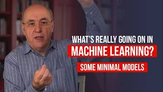
Stephen Wolfram builds minimal machine learning models from scratch to show how learning actually works. Neural nets succeed by mining the computational universe for programs that happen to work, which is why trained solutions look messy and resist explanation. Pockets of reducibility still allow for useful scientific laws.
Chapters
Hello, everyone. Well, I'm going to be talking about something that I posted at the end of last week called what's really going on in machine learning? Some minimal models. It's kind of the result of me being curious about the answer to that question for quite a long time and finally having a bit of a breakthrough and understanding it as a result of some work on biological evolution. That was kind of a surprise in terms of a discovery that I sort of didn't expect to make, that I made a few months ago. It's kind of led to some ideas about machine learning. So let me tell you what I said in the piece that I wrote. And then after I've done with that, I'll take some questions and be happy to try and provide answers. All right. The Mystery of Machine learning. It's surprising how little is known about the foundations of machine learning. Yes, from an engineering point of view, an immense amount has been figured out about how to build neural nets that do all kinds of impressive and sometimes almost magical things. But at a fundamental level, we still don't really know why neural nets work, and we don't have any kind of scientific big picture of what's going on inside them. Basic structure of neural nets can be pretty simple, but by the time they're all trained up with their weights and so on, it's been hard to tell what's going on or even to get any good visualization of it. And indeed, it's far from clear even what aspects of the whole setup are, are actually essential, and what are just details that have perhaps been grandfathered all the way from when computational neural nets were first invented in the 1940s. Well, what I'm going to try to do here is to get underneath this and to sort of strip things down as much as possible. I'm going to explore some very minimal models that, among other things, are more directly amenable to visualization. At the outset, I wasn't at all sure that these minimal models will be able to reproduce any of the kinds of things we see in machine learning. But rather surprisingly, it seems they can. And the simplicity of their construction makes it much easier to kind of see inside them and to get more of a sense of what essential phenomena actually underlie machine learning. One might have imagined that even through the training of a machine learning, even though the training of a machine learning system might be circuitous, somehow, in the end, the system would do what it does through some kind of identifiable and explainable mechanism. But what we'll see is that in fact, that's typically not at all what happens. Instead, it looks much more as if the training manages to home in on some wild computation that just happens to achieve the right results. Machine learning, it seems, isn't building structured mechanisms. Rather, it's basically just sampling from the typical complexity one sees in the computational universe to picking out pieces whose behavior turn out to overlap. What's needed, and in a sense, therefore, the possibility of machine learning is ultimately yet another consequence of my favorite phenomenon of computational irreducibility. So why is that? Well, it's only because of computational irreducibility that there's all that richness in the computational universe. And more than that, it's because of computational irreducibility that things end up being effectively random enough that that the adaptive process of training a machine learning system can reach success without getting stuck. But the presence of computational irreducibility also has another important implication, that even though we can expect to find limited pockets of computational reducibility, we can't expect kind of a general narrative explanation of what a machine learning system does. In other words, there won't be a traditional, say, mathematical general science of machine learning, or for that matter, probably also neuroscience. Instead, the story will be much closer to the fundamentally computational new kind of science that I've explored for so long, and that has brought us our physics project and the ruliad. So, in many ways, the problem of machine learning is a version of the general problem of adaptive evolution, as encountered, for example, in biology. In biology, we typically imagine that we want to adaptively optimize some overall fitness of a system. That in machine learning, we typically try to adaptively train a system to make it align with certain goals or behaviors, most often defined by examples. And yes, in practice, this is often done by trying to minimize a quantity normally called the loss. And while in biology there's a general sense that things arise through evolution, quite how this works has always been rather mysterious. But rather, to my surprise, I recently found a very simple model that seems to do well at capturing at least some of the most essential features of biological evolution. And while the model isn't the same as what we'll explore here for machine learning, it has some definite similarities. And in the end, we'll find that the core phenomena of machine learning and of biological evolution appear to be remarkably aligned and both fundamentally connected to the phenomena of computational irreducibility. So most of what I'll do here focuses on kind of foundational theoretical questions, but in understanding more about what's really going on in machine learning and what's essential and what's not. We'll also be able to begin to see how in practice, machine learning might be done differently, potentially with more efficiency and more generality. So let's start off here talking about traditional neural nets. So kind of to begin the process of understanding the essence of machine learning, let's start from a very traditional and familiar example. A fully connected multilayer perceptron neural net that's been trained to compute a certain function F of X. So let me show you that. Okay, Screen around here. Here we go. All right, so if one gives a value X at the top here, then after rippling through the layers of this network, one gets a value that almost exactly corresponds to our function F of X down here at the bottom. So if we scan through different inputs, Okay, so this is showing us how if we give a particular value X at the top here, as we ripple through the neural net, we'll get a whole sequence of different values, and the value we get at the bottom will correspond to the value of F of X for that input x. So if we scan through different inputs X, we see different patterns of intermediate values inside the network. And so here on a log scale and linear scale at the top, log scale at the bottom, here's how these intermediate values that occur in the neural net change with the input X. So the input X is on the x axis here. And what we're seeing, each curve corresponds to the way that the value of a particular artificial neuron changes in the neural net. And so this red highlighted part is the final output value. And we can see that the way that that final output value emerges looks very complicated. So how is the neural net ultimately put together? How are the values that we were plotting here determined? Well, we're using the standard setup for a fully connected multi layer network. Each node, each artificial neuron in each layer is connected to all nodes on the layer above. And the values kind of flow down from one layer to the next, being multiplied by the positive, negative or negative weight indicated by color in these pictures associated with the connection through which they flow. So the value of a given neuron is found by totaling up all of its weighted inputs from the layer before adding a certain bias value for that neuron and then applying to the result a certain nonlinear activation function here, relu or ramp, which just says if its argument is less than 0, be 0, otherwise be equal to that argument. So what overall function a given neural net will compute is determined by the collection of weights and biases that appear in the neural Net, along with its overall connection architecture and the activation function it's using. The idea of machine learning is to find weights and biases that produce a particular function that by adaptively learning from examples of that function, typically we might start from a random collection of weights, then successively tweak weights and biases to train the neural net to reproduce the function. So let's see how that works. So here we're starting at the beginning from just random weights, and we get something, a random output that really doesn't look like the function we're trying to get at all. Then we progressively train this by giving it more and more rounds of examples until eventually the weights are set up so that we exactly get the function we want. So we can get a sense of kind of how this progresses. And yes, it's complicated by plotting successive changes in individual weights over the course of the training process. The spikes that you see at the end come from kind of neutral changes that don't affect overall behavior. So the overall objective in the training is progressively to decrease the loss. In our case, the average squared difference between the true values of F of x and those generated by the neural net. The evolution of the loss defines a learning curve for the neural net. And we can see that here. And the sort of downward glitches in this learning curve correspond to points where the neural net, in effect, made a breakthrough in being able to represent our function better. So it's important to note that there's typically randomness injected into neural net training. So if one runs the training multiple times, one will get different networks and different learning curves every time. So here are some different networks that all have successfully learned this function F of X. And here are the different learning curves corresponding to those different networks. But what's really going on in neural net training? Effectively, we're finding a way to compile a function leads to some approximation into a neural net with a certain number of real value parameters. The example here, we happen to be using about 100 parameters. But what happens if we use a different number of parameters or set up the architecture of our neural net differently? So here are a few examples. So indicating that for the function we're trying to generate, the network we've been using is pretty much the smallest that will work. So, by the way, here's what happens if we change our activation function from relu, that's the sharp ramp to a smoother function called elu, which kind of has a nice curve to it. So later we'll talk about what happens when we do machine learning. With discrete systems. In anticipation of that, it's interesting to see what happens if we take a neural net of the kind we've discussed here and quantize its weights and biases in discrete levels. The result is that, as recent experience with large scale neural nets has also shown, the basic operation of the neural net does not require precise real numbers, but survives even when the numbers are at least somewhat discrete. So we see here that when the discreteness, when the discretization, the granularity is 0.0005, we still successfully produce the function. It starts to glitch out when we quantized at level 0.005, and it's seriously glitched by the time we're at 0.05, and it's just gone bonkers by the time we're quantizing the weights in steps of 0.5. So. If we can make a sort of 3D rendering of how that works as a function, that's called delta, the discreteness scale. This is showing how the function kind of survives as a more or less accurate version of the function until delta increases and at some point it loses it. Okay, so next we want to talk about simplifying the topology. Mesh neural nets. So far we've been discussing very traditional neural nets, but to do machine learning, do we really need systems that have all those details? For example, do we really need every neuron on each layer to get an input from every neuron on the previous layer? What happens if instead every neuron just gets input from at most two others, say, with the neurons effectively laid out in a simple mesh? Well, quite surprisingly, it turns out that such a network is still perfectly able to generate a function like the one we've been using as our example. And one advantage of such a mesh neural net. So what I'm showing here is a case where we've set the weights here so that we feed in a number x at the top, we get out f at the bottom, and the F of X we get out is our function here. One advantage of such a mesh neural net is that, like a cellular automaton, its internal behavior can readily be visualized in a rather direct way. So this is sort of how the mesh net generates its output. And here we are kind of stepping through different input values x and seeing for each input value x, this is how the mesh net generates its output. So you can see here the outputs are a bunch of zeros, and then it goes to 1 and back to 0 here, corresponding to the function as we feed inputs that go from whatever negative three or something up to positive three here. So we can visualize what's going on in the way that I showed before, where we look at the values, all the different values in, in this case the mesh net as a function of the input x. So hard to understand what's going on inside. And looking at these intermediate values doesn't really help much though. We can sort of see something happening in these intermediate values at places where the function F has jumps. So how do we train a mesh net on that? Basically, we can use the same procedures for a fully connected network of the kind we saw above. RELU activation functions don't seem to work well for meshnets. So so here we're going to use RELU instead. And. So this is showing the training starting from a random mesh net and progressively updating the weights. Just a thousand rounds of updating gives us a mesh net that correctly reproduces our function. So here's the actual evolution of the differences in each individual weight during the training process. So each line here corresponds to one of the positions in the mesh net, and it's showing how the value of the weight associated with that evolves through the rounds of training. Here are results for the mesh net for different seeds, and we can see they look quite different. So this is different results, random choices of how to make changes as we're doing this training. And this is the learning curves, very similar to the ones that we saw for fully connected networks above. And actually, at the size we're using, our mesh neural nets have about the same number of connections and thus weights as our example of a fully connected network. We that we looked at a few moments ago. And we see that if we try to reduce the size of our mesh neural net, it doesn't do so well at reproducing our function. So if we have a really tiny mesh neural net, this is with an LU activation function, we'll see that this is what it gets. It's a pretty coarse approximation. As we increase the size of the mesh net, we still see some glitches at this size, but by the time we're at this size here, we've accurately been able to train to reproduce our function. Okay, so. Let's go on. So now we'll talk about making everything discrete, a biological evolution analog. So mesh neural nets simplify the topology of neural net connections. But somewhat surprisingly, at first, it seems as if we can go much further in simplifying the function that's systems we're using and still successfully do versions of machine learning and in particular, we'll find that we can make our systems completely discrete. The typical methodology of neural net training involves progressively tweaking real value parameters, usually using methods based on calculus and on finding derivatives. And one might imagine that any successful adaptive process would ultimately have to rely on being able to make arbitrarily small changes of the kind that are possible with real value parameters. But in studying simple idealization of biological evolution, I recently found some striking examples where this isn't the case and where completely discrete systems seem able to capture the essence of what's going on. As an example, let's consider a three color cellular automaton. The rule is shown over here. And the behavior one generates by repeatedly applying that rule, starting from a single cell initial condition is here. The rule has the property that the pattern it generates from a single cell initial condition survives here for exactly 40 steps and then dies out so that every cell becomes white. And the important point is that this rule can be found by a discrete adaptive process. The idea is to start, say from a null rule, and then at each step to randomly change a single outcome out of the 27 in this rule here. To make that is to make sort of a single point mutation in the rule. So most such changes will cause the lifetime of the pattern to get further from our target of 40. And these we discard. But gradually we can build up kind of beneficial mutations and that through sort of this progressive adaptation, eventually get to our original lifetime 40 rule. So we can make a plot of sort of all the attempts that we made that eventually led us to the reach lifetime 14. We can think of this sort of progressive fitness curve as being directly analogous to the loss curves in machine learning that we saw before. So if we make different sequences of mutations will get different paths of adaptive evolution and different solutions for rules that have lifetime 40. But there are two things that are immediately notable about what's going on here. First, that all these different paths of adaptive evolution seem to be using different ideas to reach their goal, presumably analogous to the phenomenon of different branches in the tree of life. And second, that none of them seem to be using a clear mechanical procedure of the kind we might construct through traditional engineering to reach their goal. Instead, they seem to be finding sort of natural, complicated behavior that just happens to achieve the goal. It's non trivial, of course, that this behavior can achieve a goal like the one we've set here, as well as that simple selection based on random input, random point mutations can successfully reach the necessary behavior. But as I talked about elsewhere in connection with biological evolution, this is ultimately a story of computational irreducibility, particularly in generating diversity both in behavior and in the paths necessary to reach it. But, okay, so how does this model of adaptive evolution relate to systems like neural nets? In the standard language of neural nets, our model is like a discrete analog of a recurrent convolutional network. It's convolutional because at any given step, the same rule is applied locally throughout an array of elements. It's recurrent because, in effect, data is repeatedly passed through the same rule. The kinds of procedures like backpropagation typically used to train neural nets wouldn't be able to train such a system. But it turns out that essentially, as a consequence of computational irreducibility, the very simple method of successive random mutation can be successful. So let me talk about machine learning in discrete rules. So let's say we want to set up a system like a neural net, or at least a mesh neural net, but we want it to be completely discrete, and I mean born discrete, not just discretized from an existing continuous system. How can we do this? One approach that, as it happens, I first considered actually in the mid-1980s, but never seriously explored, is to make what we can call a rule array. Like in a cellular automaton, there's an array of rules. But instead of these cells always being updated according to the same rule, each cell at each place in the cellular automaton, analog of space time can make a different choice of what rule it will use. Although it's a fairly extreme idealization, one can potentially imagine that these different rules represent a discrete analog of different local choices of weights in a mesh neural net. As a first example, let's consider a rule array in which there are two possible choices of rules, both two color, nearest neighbor, cellular automata rules, or 146, which are respectively class two and class three. So a particular rule array is defined by which of these rules is going to be used at each space, time, position in the array. So here are a few examples. In each case, we're starting from the same single cell initial condition. But in each case, the rule array has a different arrangement of rule choices, with cells running Rule 4 being that teal color and ones running Rule 146 being that pinkish color. Well, we can see that different choices of rule array can yield different behaviors. But in the spirit of machine learning, we can, in effect, invert this and find a rule array that will give some particular behavior we want. That's what we want to do. If we're going to do machine learning with this. So a simple approach is to do the direct analog of what we did in our minimal modeling of biological evolution, Progressively make random single point mutations here, flipping the identity of just one rule in the rule array and then keeping only those mutations that don't make things worse. Just a second. So, as our sample objective, let's ask to find a rule array that makes the pattern generated from a single cell using that rule array survive for exactly 50 steps. At first, it might not seem obvious that we'd be able to find such a rule array, but in fact, our adaptive, simple adaptive procedure easily manages to do this. And we can see here that this has an infinite lifetime, this has lifetime six and so on. And we're gradually filling in, we're gradually mutating, we're flipping kind of rules in the rule array and progressively getting lifetimes that are closer to, and eventually make it to exactly 50 steps. So we can look at how did that happen. And as the dots indicate here, many mutations don't lead to longer lifetimes. But every so often, the adaptive process has a breakthrough that increases the lifetime, eventually reaching exactly 50. So, just as in our model of biological evolution, different random sequences of mutations lead to different solutions here to the problem of living for exactly 50 steps, here are a bunch of different solutions, different rule arrays that all succeed in having the single cell initial condition pattern live for exactly 50 steps. Some of these are, in effect, simple solutions that require only a few mutations, like this one here. But most, like most of our examples in biological evolution, seem more as if they just happen to work effectively by tapping into just the right fairly complex behavior. Is there a sharp distinction between these cases? Well, looking at the kind of collection of fitness curves for these examples, it doesn't really seem. So it's not too difficult to see how to construct a simple solution just by sort of strategically placing a single instance of the second rule in the rule array. Here it is. This will live for a specified number of steps. But the point is that adaptive evolution by repeated mutation normally won't discover this simple solution. And what's significant is that the adaptive evolution can nevertheless still successfully find some solution, even though it's not the one. That's one that's understandable to us. So the cellular automata rules we've been using so far take three inputs. But it turns out we can make things even simpler by just putting ordinary two input boolean functions into our rule array. For example, we can make a rule array by just using the functions and And XOR those are the R equals a half rules eight and six so different and and XOR rules show different behavior. But are there for example and and XOR rule arrays that will compute any of the 16 possible 2 input Boolean functions? We can't get not or any of the other eight other functions that map kind of white white to black or false false to true. It turns out we can get all eight functions that don't do that. And this is how we can we can do that. We're assuming the sort of the missing inputs are effectively white. So. Let's see. In fact we can also get and the nextor rule arrays to find all other even boolean functions. So for example, here are rule arrays for a couple of three input rules corresponding to the Rule 30 cellular automaton Rule 110 cellular automaton those are those Boolean functions reproduced using and plus XOR rule arrays. So it might be worth mentioning that the ability to set up such rule arrays is related to functional completeness of the underlying rules we're using. But it's not quite the same thing. Functional completeness is about setting up arbitrary formulas that that can in effect allow long range connections between intermediate results. Here all information has to explicitly flow through the array, but for example, the functional completeness of NAND allows it to generate all Boolean functions when combined. For example with first though, sometimes the rule arrays that are needed can be quite large. Okay, but what happens if we try to use our adaptive evolution process, say to solve the problem of finding a pattern that survives for exactly 30 steps? Here's a result for and an XOR ruler rays and you can see it, it overshot here a little bit and then came back. And eventually that particular pattern of ands and exors makes an initial input of a single black cell live for exactly 30 steps. Here are examples of other rule arrays that again successfully lead to patterns that live for exactly 30 steps, none of which in this case look particularly sort of mechanistic or constructed. Okay, so what about learning our original function F of X? Well, first we have to decide how we're going to represent the numbers X and F of X in our discrete rule array system. One approach is to do this simply in terms of the position of a black cell, kind of like one hot encoding. So for example, let's show an example here in this case where there's an initial black cell at a position corresponding to about x equals minus 1.1. And then the result after passing through the ROO array is a black Cell that's at the position corresponding to F of x equals 1. So now the question is whether we can find a rule array that successfully maps the initial to final cell positions according to the mapping, X goes to F of X that we want. Well, here's an example that at least comes close to doing that. We're taking the array to be cyclic here, which is why things sort of come back the other side in some cases. And sometimes we'll see that it doesn't quite nail the result. Usually it nails the result, but sometimes it just doesn't make it at all. It's kind of like a partial function. It doesn't evaluate, doesn't give any value at all here. So how did we find this? Well, we just used a simple adaptive algorithm evolution process. In direct analogy to the way it's usually done in machine learning. We set up training examples here of the form things like this. These are values of X that go to values F of X. Then we repeatedly made simple point mutations in our rule array, keeping those mutations where the total difference from all the training examples didn't increase. And after 50,000 mutations, we got the final result for the ruler array that we're showing here. So we can get some sense of kind of how we got there by showing the sequence of intermediate results where we get closer to the goal of reproducing that function, as opposed to we're showing we've kept in the adaptive evolution, we keep kind of the neutral results where we stay the same performance as before. But in this picture, we're just showing the cases where the performance improves relative to the previous picture. Okay, so here are the corresponding rule arrays that are successively that correspond to these kind of successful improvements in reproducing the function. And in each case, we're highlighting those elements of the rule array that changed from the previous iteration of the rule array, the previous version of the rule array. And we're also showing in this particular case, the computation of F of 0 to show what that does. And we'll see it's doing things, it's doing okay back here. But obviously other pieces, other values of x weren't doing okay. And so the rule array got progressively updated until eventually here they're all doing okay. So once again, an important takeaway is that we don't see identifiable mechanism in what's going on. Instead, it looks more as if the rule arrays we've got just happen to do the computations we want. Their behavior is complicated, but somehow we managed to tap into it, to compute our f of X. But how robust is this computation? Well, a key feature of typical machine learning is that it can generalize away from the specific examples it's been given. It's never been clear just how to characterize that generalization when there's an image of a cat in a dog suit start being identified as an image of a dog. But at least when we're talking about classification tasks, we can think of what's going on in terms of basins of attraction that lead to attractors corresponding to our classes. It's all considerably easier to analyze, though, in the kind of discrete system we're exploring here. For example, we can readily enumerate all our training inputs, that is all initial states containing a single black cell, and then see how frequently these cause any given cell to be black. Let's see. Here we go. And so this is kind of showing superimposing all of our examples. Let's see. This is what happens if we make this plot at each of the successive breakthroughs during training. This is showing how the kind of the overall set of excitations of the network gradually correspond. Gradually correspond better to getting the final function. So what happens if this is the case where we're looking at sort of valid inputs, where we just have a single black cell in the input? What about all possible inputs, including ones that don't just contain a single black cell? Well, because this is a discrete system, we can enumerate all of them and compute the overall frequency for each cell in the array to be black. This is now not just the valid inputs that correspond to a single black cell, but all possible inputs. So, as we might expect, the result is sort of considerably fuzzier than what we got purely with our training inputs. But there's still a strong trace of the discrete values of F of x that appeared in the training data. If we plot the overall probability for a given final cell to be black, we see here peaks at the positions corresponding to the value 0 and 1 that F of x takes on. So this is now plotting the probability on a large scale, the probability to get a certain output value. And we see that the vastly overwhelming likelihood is that we'll get 1 of the output values that correctly corresponds to an output to the function. Okay, so because our system is discrete, we can just look at explicitly at all possible outcomes that occur. Funny quotes at the top here. And we can see that the most common overall from all possible, including meaningless inputs, is the meaningless sort of all white state. That basically happens when the computation never makes it to the output. But the next most common outcomes correspond exactly to F of x equals 0 and f of x equals 1. After that is a kind of superposition outcome where F of x is in effect both 0 and 1. But okay, so what initial states are in the basins of attraction of that is will evolve to the various outcomes here. The failure plots, fairly flat plots here, indicate that the overall density of black cells gives very little information about what attractor a particular initial state will evolve to. So this means we have to look at specific configurations of cells in the initial conditions. So as an example, let's say we start from this initial condition which evolves to this final condition. Now we can ask what happens if we look at a sequence of slightly different initial conditions. So here we're showing kind of in black and white initial conditions that still evolve to the original attractor state and in pink ones that evolve to some different state. So, well, what's actually going on inside here? This is all a bit complicated. Here are a few examples kind of highlighting cells whose values change as a result of changing the initial condition. So as is typical in machine learning, there doesn't seem to be any simple characterization of the form of the basin of attraction. But now we have a sense of what the reason for this is. It's another consequence of computational irreducibility. Computational irreducibility gives us the effective randomness that allows us to find useful results by adaptive evolution. But it also leads to changes having what seem like random and unpredictable results. Worth noting, by the way, that we could probably dramatically improve the robustness of our attractor basins by specifically including our training data examples, including training data examples that have kind of noise injected. All right, let's go on here. We're going to talk now about multi way mutation graphs. So in doing machine learning in practice, the goal is typically to find some collection of weights and so on that successfully solve a particular problem. But in general, there will be many such collections of weights. With typical continuous weights and random training steps, it's very difficult to see the whole ensemble of possibilities. But in our discrete rule array systems this becomes more feasible. So let's consider a tiny two by two rule array with two possible states. Two possible rules. Sorry. We can make a graph whose edges represent all possible point mutations between those rule arrays. So in our adaptive evolution process, we're always moving around a graph like this. But typically most moves will end up in states that are rejected because they increase whatever loss we've defined. So consider the problem of generating an and and plus XOR rule array in which we end with lifetime four patterns. Defining the loss as how far we are from this lifetime, we can draw a graph that shows all possible adaptive evolution paths that always progressively decrease the loss. The result here is a multi way graph of the type we've now seen in a great many kinds of situations, notably our recent study of biological evolution. Although this particular example is quite trivial, the idea in general is that different parts of such a graph represent different strategies for solving a problem. In direct analogy to our physics project and our studies of things like game graphs, one can imagine such strategies being laid out in a branchial space defined by common ancestry of configurations. In the multi way graph, one can expect that while in some cases the branchial graph will be fairly uniform, in other cases it will have quite separated pieces that represent fundamentally different strategies. Of course, the fact that underlying strategies may be different doesn't mean that the overall behavioral performance of the system will be noticeably different. And indeed, one expects that in most cases, computational irreducibility will lead to enough effective randomness that there'll be no discernible difference. But in any case, here's an example starting with a rule array that contains both and an xor, where we observe distinct branches of adaptive evolution that lead to different solutions to the somewhat trivial problem of finding a configuration of this rule array with a lifetime of exactly four. And those solutions are highlighted here. Okay, let's talk about optimizing the learning process. How should one actually do the learning in machine learning? In practical work with traditional neural nets, learning is normally done using systematic algorithmic methods like backpropagation. But so far all we've done here is something much simpler. We've learned by successfully making random point mutations and keeping only ones that don't lead us further from our goal. And yes, it's interesting that such a procedure can work at all. And as we've discussed elsewhere, this is presumably very relevant in understanding phenomena like biological evolution. But as we'll see, there are more efficient, and probably much more efficient methods of doing machine learning, even for the kinds of discrete systems that we're studying here. So let's start by looking again at our earlier example of finding an and an XOR rule array that gives a lifetime of exactly 30. So at each step in our adaptive learning process, we make a single point mutation, changing a single rule in the rule array, keeping the mutation. If it doesn't take us further from our goal, the mutations gradually accumulate, every so often reaching a rule array that gives a lifetime closer to 30. So just as above, here's a plot again of the lifetime achieved by successive mutations with these sort of internal red dots here corresponding to rejected mutations. So we see a series of plateaus at which mutations are accumulating but not changing the overall lifetime. And between these, we see occasional breakthroughs where the lifetime jumps. So here are the actual rule array configurations for these breakthroughs with mutations since the last breakthrough highlighted. But in the end, the process here is quite wasteful. In this example, we make a total of 1705 mutations, but only 780 of them actually contribute to generating the final rule array. All the others are discarded along the way. So how can we do better? One strategy is to try to figure out at each step which mutation is most likely to make a difference. And one way to do that is to try every possible mutation in turn at every step, as in multi way evolution, and see what effect each of them has on the ultimate lifetime. So from this we can kind of construct a change map in which we give the change of lifetime associated with mutation at every particular cell. The results will be different for every configuration of a rule array of I. E. At every step in the adaptive evolution. But for example, here's what they are for a particular for, for the particular breakthrough configurations that we were just looking at here. And so the elements that are colored gray don't affect the results if they're changed. The ones colored red have a positive effect, with more intense red being more positive, and the ones colored blue have a negative effect. So let's start, say we start from a random rule array, then repeatedly construct the change map and apply the mutation that it implies gives the most positive change in effect at each step, following the path of steepest descent to get to the lifetime we want, that is to reduce the loss. Then the sequence of breakthrough configurations that we get is this. So this is in effect a slightly more direct path to a solution than our sequence from pure single point mutations. By the way, the particular problem of reaching a certain lifetime has a simple enough structure that this steepest descent method, when started from a simple uniform rule array, finds a very mechanical, if slow, path to a solution. Here it is. So what about the problem of learning our F of x function that we had before? Once again, we can make a change map based on the loss. We define here the results for a series of breakthrough configurations. The gray regions are ones where the changes will be neutral. So there's still exploration that can be done without. There can be done without affecting the loss. The red regions are ones that are in effect locked in and where Any changes will be deleterious in terms of loss. So what happens in this case if we follow the path of steepest descent, always making the change that will be best according to the change map? Well, the results are actually. What's this? That's. The results turn out to be actually quite unsatisfactory. From almost any initial condition, system quickly gets stuck, never finds any satisfactory solution. In effect, it seems that deterministically following the path of steepest descent leads us to a local minimum from which we can't escape. So what are we missing in just looking at the change map? Well, the change map as we've constructed it has the limitation that it's separately assessing the effect of each possible individual mutation. It doesn't deal with multiple mutations at a time, which could well be needed in general if one's going to find the fastest path to success and avoid getting stuck. But even in constructing the change map, there's already a problem, because at least the direct way of computing it scales quite poorly. In an n by n rule array. We have to check, in effect, the effect of flipping about n squared values. And for each of these, we have to run the whole system altogether, taking about N to the fourth operations. One has to do this separately for each step in the learning process. So how do traditional neural nets avoid this kind of inefficiency? The answer, in a sense, involves a mathematical trick, at least as it's usually presented. It's all based on the continuous nature of the weights and values in neural nets, which allow us to use methods from calculus. So let's say we have a neural net like this that computes some particular function F of X. Like this. We can ask how this function changes as we change each of the weights in the network. In effect, this gives us something like our change map from above. But there's an important difference. Because the weights are continuous, we can think about infinitesimal changes to them. And then we can ask questions like how does F of x change when we make an infinitesimal change to a particular weight? Let's say the weight here, the. Or equivalently, what is the partial derivative of F with respect to. With respect to some weight W sub I at a particular point x. So then now we get to use a. So this is what this is showing. This is. This is a weight W sub I, and this is the change in the value of F as a function of X associated with an infinitesimal change. Each of these different curves corresponds to a slightly different value for W sub I for that weight so we get to use a sort of key feature of infinitesimal changes that they can always be thought of as sort of just adding linearly, because essentially epsilon squared can always be ignored compared to epsilon when epsilon is sufficiently infinitesimally small. Or in other words, we can summarize any infinitesimal change just by giving its direction in weight space, that is a vector that says how much of each weight should be infinitesimally changed. So if we want to change F of x infinitesimally as quickly as possible, we should go in the direction of steepest percent, defined by all the derivatives of F with respect to the weights. So in machine learning, we're typically trying, in effect, to set the weight so that the form of F of X we generate successfully minimizes whatever loss we've defined. And we do this by incrementally moving in weight space at every step, computing the direction of steepest descent to know where to go next. In practice, there are all sorts of tricks like ADAM that try to optimize the way to do this. But how do we efficiently compute the partial derivative of F with respect to each of these weights? In our case, yes, we could do the analog of generating pictures like the ones above. Sorry, how do we efficiently compute this partial derivative with respect to each of the weights? We could do the analog of these pictures here separately for each of the weights. But it turns out that there's a standard result from calculus that gives us a vastly more efficient procedure that in effect maximally reuses the parts of the computation that we've already done. It all starts with the textbook chain rule. The derivative of nested, I.e. composed functions so basically says that the infinitesimal change in the value of the whole chain D of C of B of A of X can be computed as a product of infinitesimal changes associated with each of the links in the chain. But the key observation is then that what we get when we, when we get to the computation of the change at a certain point in the chain, we've already had to do a lot of the computation we need. And so long as we stored those results, we always have only an incremental computation to perform. So how does this apply to neural nets? Well, each layer in a neural net is in effect doing a function composition. So, for example, our C of B of A of X is like kind of a trivial neural net here. But what about the weights, which, after all, are what we're trying to find the effect of changing? Well, we can include them explicitly in the function we're computing like this, then we could in principle, symbolically compute the derivatives with respect to these weights. There are derivatives with respect to each of those weights. And for the network here that we had, this corresponds to the corresponding expression. Ignoring biases is this where phi is the activation function. So once again, we're dealing with nested functions. And once again, though it's a bit more intricate. In this case, the computation of derivatives can be done by incrementally evaluating terms in the chain rule, in effect using the standard neural net method of backpropagation. So what about the discrete case? Are there similar methods we can use there? Well, let's not discuss this in detail here, but we'll give some indications of what's likely to be involved. As a potentially simpler case, let's consider ordinary cellular automata. The analog about change maps asks how the value of a particular output cell is affected by changes in other cells, or in effect, what the partial derivative of the output value is with respect to changes in values of other cells. For example, let's consider kind of the highlighted output cell in this cellular automaton evolution. Now we can look at each cell in this array and make a change map based on seeing whether flipping the value of just that cell and then running the cellular automaton forwards from that point would change the value of the highlighted output cell. So this is the the change map that we get. In that way, the form of the change map is different if we look at different output cells. And here, by the way, are some larger change maps for this and a couple of other cellular automaton rules. But is there a way to construct such change maps incrementally? One might have thought that there would immediately be, at least for cellular automata, that, unlike cases here, are fundamentally reversible, that there will be such an incremental way to compute the change map. But actually, such reversibility doesn't seem to help much, because although it allows us to backtrack whole states of the cellular automaton, it doesn't allow us to trace the separate effects of individual cells. How about using discrete analogs of derivatives in the chain rule? Let's, for example, call the function computed by one step in Rule 30, cellular automaton evolution W of X, Y and Z. We can think of the partial derivative of this function with respect to X at the point X as representing whether the output of W changes when X is flipped. Starting from value given, I shouldn't have used the W as the symbol for this. It confuses it with weights this is the actual value of the soil of Taunton. So what we're doing here is we have the function that's value of the cellular automaton. Then we're asking whether there's a change when we change the X, which is the left hand cell value. So no change is indicated as false or white cell, while a change is indicated as true or a black cell. And yes, one can either explicitly compute the rule outcomes here and then deduce from them the functional form, or one can use symbolic rules to directly deduce the functional form which we're showing over here. So one can compute a discrete analog of a derivative for any Boolean function. So for example, we have strange formulas like this and a formula like that. The derivative of xor is not. And we could also write that in this way here the derivative of this explicitly written out rule is another explicitly written out rule. And we have all sorts of other curious relations here that are the discrete analog of calculus now applied to Boolean functions. Actually, here's a table of Boolean derivatives for all two input Boolean functions. And there's indeed a whole Boolean calculus one can set up for these kinds of derivatives. And in particular there's a direct analog of the chain rule where xnor is effectively the equality test. Does X equal y? Okay, but so how do we use this to create our change maps? In our simple cellular automaton case, we can think of our change map as representing how a change in an input cell propagates back to previous cells. But if we just try to apply our discrete calculus rules, we run into a problem. Different chain rule chains can imply different changes in the value of the same cell. In the continuous case, this path dependence doesn't happen because of the way infinitesimals work, but in the discrete case it does. And ultimately we're doing a kind of backtracking that can really be represented faithfully only as a multi way system. Though if we just want probabilities, for example, we can consider averaging over branches of the multi way system. And the change maps we showed above are effectively the result of thresholding over the multi way system. But despite the appearance of such difficulties in the simple cellular automaton case, such methods typically seem to work better. In our original, more complicated rule array case, there's a bunch of subtlety associated with the fact that we're finding derivatives not only with respect to the values in the rule array, but also with respect to the choice of rules, which are the analog of weights in the continuous case. So let's Consider an and and XOR rule array. Here our loss is the number of cells whose values disagree with the row shown at the bottom with with this cell here. So now we can construct a change map for this rule array both in a direct forward way by just seeing what the result is from changing each each value, each rule array element, and backwards using our discrete derivative methods, where we effectively resolve the small amount of multi way behavior by always picking majority values. So this is the result from that by direct forward computation and by this backward computation. So the results are similar, though in this case not exactly the same. So here are a few other examples and yes, in detail, there are essentially always local differences between the results from the forward and backward methods. But the backward method, like in the case of backpropagation in ordinary neural nets, can be implemented much more efficiently. And for purposes of practical machine learning, it's actually likely to be perfectly satisfactory, especially given that the forward method is itself only providing an approximation to the question of which mutations are best to do. So, as an example, here are some results from forward and backward methods for the problem of computing of learning the function F of x that we've talked about, again shown for the breakthrough configurations that we looked at above. Okay, let's talk about what can be learned. So we've now seen quite a few examples of machine learning in action. But a fundamental question we haven't yet addressed is what kind of thing can actually be learned by machine learning? Even before we get to this, there's another question. Given a particular type of system, what kinds of functions can it even represent? As a first example, let's consider a minimal neural net of essentially this form, essentially a single layer perceptron network. And with the RELU activation function AKA ramp, the first set of weights, and the first set of weights here taken to be one, as in this picture here, the function computed by a neural net like this has this mathematical form. So turns out with enough weights and biases, this form can represent any piecewise linear function. So for example, this essentially just by moving around ramps and using biases and scaling them using weights. So for example, if we look at this function here, This is the function that's computed by that neural net that I just showed here. And here's how that function is kind of built up by adding in successive ramps associated with individual intermediate nodes or neurons. So it's similarly possible to get all smooth functions from activation functions like elu and so on. Things get more complicated if we try and represent functions with more than one argument With a single intermediate layer, we can only get sort of Piecewise hyperplanar functions, I.e. functions that change direction only at linear fault lines. But already with two intermediate layers and sufficiently many nodes in each of these layers, we can generate any piecewise function of any number of arguments. If we limit the number of nodes, then roughly we limit the number of boundaries between different linear regions and the values of the functions. But as we increase the number of layers with a given number of nodes, we basically increase the number of sides that political regions within the function values can have. So here are some examples of what functions we can compute. These are now functions of two inputs Here. Let's say X and Y. And this is the values F of X and Y shown from these networks. What happens with the mesh nets that we looked at before? Well, here are a few random examples of mesh nets showing results that are very similar to shallow fully connected networks with a comparable total number of nodes. So how about our fully discrete rule arrays? What functions can they represent? We already saw part of the answer earlier when we generated rule arrays to represent various Boolean functions. It turns out that there's a fairly efficient procedure that based on boolean satisfiability, we're explicitly finding rule arrays that can represent a given function or determine that no rule array, say, of a given size can do this. So using this procedure, we can find minimal and an XOR rule arrays that represent all even three input boolean functions, that is all R equals one cellular automaton rules. So here they are. So it's, it's always possible to specify any n input boolean function by an array of two to the n bits. But we can see from these pictures that when we compile Boolean functions into and an XOR rule arrays, they can take different numbers of bits, that is different numbers of elements in the rule array. So in effect, the algorithmic information content of the function varies with the language we're using to represent them. So for example, in the case we're looking at here with three input Boolean functions, the distribution of minimal rule array sizes is this. There are some functions that are more difficult to represent as and XOR rule arrays and seem to require like 15 ruler elements and others that are easier. This is similar to what happens if we represent Boolean functions as Boolean expressions saying conductive, normal form and count the total number of unary and binary operations used. Okay, so we know that there is in principle an and an XOR rule array that will compute any even Boolean function. So now we can ask whether an adaptive evolution process can actually find such a rule array, say, with a sequence of single point mutations. Well, if we do such adaptive evolution with a loss that counts the number of wrong outputs for, say, Rule 254, then here's the sequence of successive breakthrough configurations that are produced. So here what we're showing, every row shows all the possible inputs and shows the outcomes that we get. And so on the final row we get the correct sequence of outcomes that corresponds to the final kind of breakthrough configuration of arranging the rule array. And earlier on, when we've got very few XORs in the rule array, it doesn't do very well at computing this. We need this whole mixture of ands and xors to do this computation. So the results here are not as compact as the minimal solution. If we go back here, we can see somewhere here the minimal solution for Rule 254. It's down in the corner there, and it's a bit smaller than what we've got got here. So. What's interesting is that even though it's not as compact as the minimal solution that we could find by exhaustively searching all possibilities, it seems to always be possible to at least find some and XOR rule array that solves the problem just by using adaptive evolution with single point mutations. So here are results for a few other boolean functions showing kind of on the top row of each of these, showing the sequence of breakthrough configurations and the bottom kind of proving that it works by looking at all the possible inputs. So yes, not only are all even boolean functions representable in terms of and and XOR rule arrays, they're also learnable in this form just by adaptive evolution with single point mutations. So in what we were doing before, we were looking at how machine learning works with our rule arrays in specific cases, like for our F of x function. But now we've got a case where we can explicitly enumerate all possible functions, at least of a given class. In a sense, what we're seeing is evidence that machine learning tends to be very broad and capable, at least in principle, of learning pretty much any function. Of course, there can be specific restrictions like the and and XOR rule arrays we're using here can't represent odd functions where, you know, white plus white goes to black and so on. The NAND plus first rule arrays we discussed above can do that case. But in general, it seems to be a reflection of the principle of computational equivalence that pretty much any setup is capable of representing any function and also adaptively learning it, by the way, it's a lot easier to discuss questions about representing or learning any function when one's dealing with discrete countable functions, because one can expect to either be able to exactly get a given function or not. For continuous functions, it's much more complicated because one's pretty much inevitably dealing with approximations. And thus one can use symbolic forms which are basically discrete. So, for example, while we can say, as we did above, that RELU neural nets can represent any piecewise linear function, in general, we'll only be able to imagine successively approaching an arbitrary function, much like when you kind of add progressively more terms in a simple Fourier series. Okay, so looking. Thinking back to our results for discrete ruler arrays, one notable observation is that while we can successfully reproduce all these different Boolean functions, the actual rule array configurations that achieve this tend to look quite messy. And indeed, it's much the same. As we've seen throughout here, machine learning can find solutions, but they're not structured solutions. They're in effect, just solutions that happen to work. So are there more structured ways of representing Boolean functions with rule arrays? So here are sort of two possible minimum size and the nexor rule arrays that represent Rule 30. At the next larger size, there are more possibilities for Rule 30. And there are also rule arrays that can represent Rule 110. All of these can represent Rule 110. But in none of these cases is there obvious structure that allows us to immediately see how these computations work or what function is being computed. But what if we try to explicitly construct, essentially by standard engineering methods, a rule array that computes a particular function? We can start by taking something like the function for Rule 30 and writing it in terms of and an XOR that is in ANF or algebraic normal form. So this is. That's the Rule 30 function in ANF. We can imagine implementing this using an evaluation graph. Here it is. But now it's easy to turn this into a rule array. And yes, we haven't gone all the way here and arranged to do things like copy inputs, which is what those previous rule arrays did manage to do. So evaluating this rule array for different inputs, we find that it indeed gives Rule 30 doing the same thing for Rule 110. The and XOR expression is this, the evaluation graph is this, and the rule array is this. And at least with the evaluation graph as a guide, we can readily sort of see what's happening here. But the rule array we're using is considerably larger than our minimal solutions that we have had before or even than the solutions we found by adaptive evolution. And this doesn't even solve the problem of copying initial variables, and so on. So it's a typical situation that one sees in many other kinds of systems, like for example, sorting networks. It's possible to have a constructed solution that has clear structure and regularity and is understandable. But minimal solutions, or ones found by adaptive evolution tend to be much smaller. But they also almost always look in many ways random and aren't readily understandable or interpretable. So so far we've been looking at rule arrays that compute specific functions. But in getting a sense of what rule arrays can do, we can consider rule arrays that are programmable in that their input specifies what function they should compute. So here, for example, is an and and XOR rule array found by adaptive evolution that takes the bit pattern of any even Boolean function as input should have said on the right here, then applies that Boolean function to the inputs on the left. And with this rule array we can now compute any possible even boolean function. So here's this rule array evaluating or given the rule table effectively for or fed in as input. Okay, let me talk about other kinds of models and setups. So our general goal here has been to set up models that capture most essential features of neural nets and machine learning, but that are simple enough in their structure that we can readily look inside and get a sense of what they're doing. Mostly we've concentrated on rule arrays as a way to provide a minimal analog of standard sort of perceptron style feed forward neural nets. What about other architectures and setups? Well, in effect, our rule arrays are space time inhomogeneous generalizations of cellular automata in which adaptive evolution determines which rule, say, from a finite set should be used at every spatial position and every time step a different idealization. In fact, we already used above before is to have an ordinary homogeneous cellular automaton, but with a single global rule determined by adaptive evolution. So rule arrays are the analog of feedforward networks in which a given rule in the rule array is in effect used only once as data flows through the system. Ordinary homogeneous cellular automata are like recurrent networks in which a single stream of data is in effect subjected over and over again to the same rule. There are various interpolations between these cases. For example, we can imagine a layered rule array in which rules at different steps can be different, but those on a given step are all the same. So a system like this can be viewed as an idealization of a convolutional neural net in which a given layer applies the same kernel to all unlets at all positions, but different layers can apply different kernels. A layered rule can't encode as much information rule array, rather than encode as much information as a general rule array, but it's still able to show machine learning style phenomena. And so here, for example, there's an adaptive evolution of a layered and plus xor rule array that progressively solves the problem of generating a pattern that lives for exactly 30 steps. So one could also imagine vertically layered rule arrays, in which different rules are used at different positions, but any given position keeps running the same rule forever. However, at least for the kinds of problems we've considered here, it doesn't seem sufficient to just be able to pick the positions at which different rules are run. One seems to either need to change rules at different time steps, or one needs to be able to adaptively evolve the underlying rules themselves. Okay, so rule arrays and ordinary cellular automata share the feature that the value of each cell depends only on the values of neighboring cells on the step before. But in neural nets, it's standard for the value at a given node to depend on the values of lots of nodes on the layer before. And what this makes this straightforward in neural nets is that weighted and perhaps otherwise transformed values from previous nodes are taken to be combined by simple numerical addition. And addition, being nary and associative, can take any number of inputs. In a cellular automaton or Boolean function, there's always a definite number of inputs determined by the structure of the function. The most straightforward case, the inputs come only from nearest neighboring cells. But there's no requirement that this is how things need to work. And for example, we can pick any local template to bring in the inputs for our function. This template could either be the same at every position at every step, or it could be picked from a different set differently at different positions, in effect giving us template arrays as well as rule arrays. So what about having a fully connected network, as we did in our first neural net examples above? So, to set up a discrete analog of this, we first need some kind of discrete NRE associative accumulator function to fill the place of numerical addition? And for this we could pick a function like and, or xor or majority. And if we're not just going to end up with the same value at each node on a given layer, we need to set up some analog of a weight associated with each connection, which we can achieve by applying either identity or not that is flip or not to the value flowing through each connection. So here's an example of this kind of network trained in this case to compute our function F of X. There are just two kinds of connections here. Flip which is I think blue or don't flip which is I think red. And at each node we're computing the majority function, in other words, giving 1 if the majority of the inputs are 1 and 0 otherwise. So with the 1 hot encoding of input and output that we used before for our function F of X, here are some examples of how this network evaluates our function. So, remembering that the value of X is determined by which cell was black on the initial state and the value of F of X by which cell is black on the final state. So. This particular setup was trained using just 1000 steps of single point mutation applied to the connection types. The loss systematically goes down, but the configuration of the connection types continues to look quite random even as it achieves zero loss, that is even after the function has been completely learnt. So this is a picture of. This is a picture of the actual values of the kind of the weights, the flip or no flip. And that's a picture of the loss as a function of number of, of rounds of training. So in what we've done so far, we assume that all connections continue to be present, though their types are effectively signs can change, but we can also consider a network where connections can end up being zeroed out during training, so they're effectively no longer present. Okay, but much of what we've done here with machine learning has centered around trying to learn transformations of the form X goes to F of X. But another typical application of machine learning is auto encoding, or in effect, learning how to compress data representing a certain set of examples. And once again, it's possible to do such a task using rule arrays with learning achieved by a series of single point mutations. So, as a starting point, consider training a rule array of cellular automaton rules 4 and 146tr to produce unchanged, reproduce unchanged, a block of black cells of any width. So one might have thought that this would be trivial, but it's not, because in effect, the initial data inevitably gets ground up inside the rule array and has to be reconstituted at the end. But nevertheless, it's possible to train a ruler array to at least roughly do this. So we're seeing the block, the black block at the beginning is more or less reconstituted at the end by going through the same rule array in all cases. But the rule arrays that do this once again end up looking quite random. To set up a non trivial autoencoder, let's imagine that we progressively squeeze this array in the middle, creating an increasingly narrow bottleneck in which the data has to flow. At the bottleneck, we effectively have a compressed version of the original data. And we find that at least down to some width of bottleneck, it's possible to create rule arrays that with reasonable probability can act as successful autoencoders of the original data. So the success of LLMs has highlighted the use of machine learning for sequence continuation and the effectiveness of transformers for this. Just as with other neural nets, the forms of transformers that are used in practice are typically very complicated. But can one find a minimal model that nevertheless captures the essence of transformers? Let's say we have a sequence. We want to continue like this. We want to encode each possible value here by a vector, as in something like this. So that, for example, our, this is how our initial sequence. Let me see, do I have one here? Yes, this is how our initial sequence is encoded in terms of these vectors here that represent particular values effectively of F of X. So then let's say we have a head that reads a block of consecutive vectors, picking off certain values, feeding pairs of them into and. And XOR functions to get a vector of boolean values. So here's how that works. We've got this kind of head that's sampling our blocks of vectors in particular places, then feeding those sampled values. You can see that white value getting fed in here to this. Is that an and an Xor? I've forgotten to this. And let's say. Actually we should have made on the outside here. We should have shown what the outputs for the. Oh no, we do. We're showing. This is an output. This is. Right, this is, this is. This is a one output. And this is a. Sorry, this is a zero output. This is a one output. This sample, these values here and here brought them together. And this is a darkened kind of reddish thing representing A1 from that, from that XOR there. Although that's an and. I think actually we can see whether it's an and or an xor. And it's clearly an XOR because it's got one black and one white. Anyway, so ultimately this head is kind of going to slide along our sequence, predicting what the next element in the sequence will be. But somehow we have to go from our vector of boolean values here to probabilities of sequence elements. Potentially we might be able to do this just with a rule array but for our purposes here, we'll use a fully connected single layer identity plus not network in which each output node just find the sum of the number of values that come to it and treat this as determining through a softmax the probability of the corresponding element. So this is how that works for that we're taking those values coming out of those Xor and ands and we're putting them through this fully connected network. And then we're saying, you know, what's the, what's, what's the winning value here? Which in this case would be the six here. And okay, so the maximum value is this, this maximum value here is a six. But this occurs for element five. So kind of at zero temperature. This will be our best prediction for the next element in this predicted by the system. So to train this whole system we just make a sequence of random point mutations to everything, keeping mutations that don't increase the loss. Well, the loss is basically the difference between the predicted next values and actual next values, or more precisely the categorical cross entropy. So here's how this loss progresses in a typical neural net training. Sorry, in a typical, in a typical training, this is not a neural net. This is a very discretized analog of a neural net. So at the end of the training, here are the components in our sort of minimal transformer. It's a very artist's impression of a transformer cartoon of a transformer. So first come the encodings of the different possible elements in the sequence. Then there's the head. And this is shown applied to the encoding of the first elements in the original sequence. From there there's a single layer discrete network that takes the output from the head and deduces relative probabilities. Or over here, sorry, this is a single layer discrete network that deduces relative probabilities. That's based on sort of summing up how many flip versus non flip connections there were to ones versus zeros here. And it deduces relative probabilities for different elements. In this case, the highest probability prediction for the next element is that it should be element. No, it shouldn't be element 10. That's element 1, 2, 3, 4, 5. We should label these with the of lay things on the right. And let's see. So this is. Yeah, it should be element six because we're going here from the bottom. So that's the highest value from the neural net. And the position of that highest value is position 6. So that's the prediction for what the next element should be of our sequence. So to do the analog of an LLM. We start from some initial prompt, that is an initial sequence that fits within the width, the context window of the head. Then we progressively apply our kind of minimal transformer, for example, at each step, taking the next element to be the one with the highest predictive probability that is operating at zero temperature. So with this setup, the collection of prediction strengths is shown in gray here, with the best prediction shown in red. So we're winners here, running this even far beyond our original training data. That was our original training data. There we see that we get a prediction of the continued sine wave. That's our highest probability prediction. Well, as we might expect, the fact that our minimal transformer can make such a plausible prediction relies on the simplicity of our sine curve. If we use more complicated training data, like a mathematically defined sine x plus sine square root of 2x curve here. Let's see. Oh, that's sort of, that's a continuation of the sine curve. That's great. But this is now our sine x plus sine root 2x, showing the part we're going to train on and the part that we want to predict in blue at the beginning and a yellow at the end. So the result of training and running our sort of minimal transformer is now this. So we see that in the region where it's been trained, it had training data. It does just fine in the region where it's kind of predicting for itself. It's really crummy. And not surprisingly, it sort of can't figure out the computation to correctly continue the curve. By the way, different training runs will involve different sequences of mutations, will lead different predictions. Sometimes it'll have a kind of periodic hallucination, like in this case here. Okay, so in looking at kind of perceptron style neural nets, we wound up using rule arrays, or in effect, space time inhomogeneous cellular automata as our minimal models. Here we've ended up with a slightly more complicated minimal model for transformer neural nets. But if we were to simplify it further, we would end up with not with something like a cellular automaton, but but instead with something like a tag system in which one has a sequence of elements and at each step removes a block from the beginning and depending on the form that one has, adds a block to the end, as shown with these rules down here. And so with even a very simple system like this, one can generate extremely complex behavior, reinforcing the idea that we've repeatedly seen here that we machine learning works by selecting complexity that aligns with the goals that have been set. And along these lines, one can consider all sorts of different computational systems as foundations for machine learning. Here we've been looking at cellular, automaton like and tag system like examples. But for example, our physics project has shown us the power and flexibility of systems based on hypergraph rewriting. And from what we've seen here, it seems very plausible that something like hypergraph rewriting can serve as a yet more powerful and flexible substrate for machine learning. Okay, so in the end, what's going on in machine learning? There are, I think, several quite striking conclusions from what we've been able to do here. The first is just that models much simpler than traditional neural nets seem capable of capturing the essential features of machine learning. And indeed, these models may well be the basis for a new generation of practical machine learning. But from a scientific point of view, one of the things that's important about these models is that they're simple enough in structure, and that it's immediately possible to produce visualizations of what they're doing inside. And studying these visualizations, the most immediately striking feature is how complicated they look. It could have been that machine learning would somehow crack systems and find simple representations for what they do. But that doesn't seem to be what's going on at all. Instead, what seems to be happening is that machine learning is, in a sense, just hitching a ride on the general richness of the computational universe. It's not specifically building up behavior one needs, but rather it's doing. What it's doing is to harness behavior that's already out there in the computational universe. So the fact that this could possibly work relies on the crucial and at first unexpected fact that in the computational universe, even very simple programs can ubiquitously produce all sorts of complex behavior. And the point is then that this behavior has enough richness and diversity that it's possible to find instances of it that align with machine learning objectives once defined. In some sense, what machine learning is doing is to mine the computational universe for programs that do what one wants. And it's not that machine learning nails a specific, precise program. Rather, it's that in typical successful applications of machine learning, there are lots of programs that do more or less the right thing. If what one's trying to do involves something computationally irreducible, machine learning won't typically be able to get well enough aligned to correctly get through all the steps of the irreducible computation. But it seems that many human like tasks that are the particular focus of Modern machine learning can successfully be done. And by the way, one can expect that with the minimal models explored here, it becomes becomes more feasible to get a real characterization of what kinds of objectives can successfully be achieved by machine learning and what cannot. Critical to the operation of machine learning is not only that there exist programs that can do particular kinds of things, but also that they can realistically be found by adaptive evolution processes. So in what we've done here, we've often used what's essentially the very simplest possible process for adaptive evolution, a sequence of point mutations. What we've discovered is that even this is usually sufficient to lead us to satisfactory machine learning solutions. It could be that our paths of adaptive evolution would always be getting stuck and not reaching any solution. But the fact that this doesn't happen seems critically connected to the computational irreducibility that's ubiquitous in the systems we're studying. And that leads to effective randomness that with overwhelming probability, will, will give us a way out of anywhere where we got stuck. In some sense, computational irreducibility levels the playing field for different processes of adaptive evolution and lets even simple ones be successful. Something similar seems to happen for the whole framework we're using. Any of a wide class of systems seem capable of successful machine learning, even if they don't have the detailed structure of traditional neural nets. We can see this as a typical reflection of the principle of computational equivalence, that even though systems may differ in their details, they're ultimately all equivalent in the computations that they can do. The phenomenon of computational irreducibility leads to a fundamental trade off, of particular importance in thinking about things like AI. If we want to know in advance, to be able to know in advance and broadly guarantee what a system is going to be able to do, we have to set the system up to be computationally reducible. But if we want the system to be able to make the richest use of computation, it'll inevitably be capable of computationally irreducible behavior. And it's the same story with machine learning. If we want machine learning to be able to do the best it can, and perhaps give us the impression of achieving magic, then we have to allow it to show computational irreducibility. And if we want machine learning to be understandable, it has to be computationally reducible and not except able to access the full power of computation. At the outset, though it's not obvious whether machine learning actually has access to such power. It could be that there are computationally reducible ways to solve the kinds of problems we want to use machine learning to solve. But what we've discovered here is that even in solving very simple problems, the adaptive evolution process that's at the heart of machine learning will end up sampling and using what we can expect to be computationally irreducible processes. Like biological evolution. Machine learning is fundamentally about finding things that work without the constraint of understandability that's forced on us when we as humans explicitly engineer things step by step. Could one imagine constraining machine learning to make things understandable? To do so would effectively prevent machine learning from having access to the power of computationally irreducible processes. And from the evidence here, it seems unlikely that with this constraint, the kind of successes we've seen in machine learning would be possible. So what does this mean for the science of machine learning? One might have hoped that one will be able to look inside machine learning systems and get detailed narrative explanations for what's going on that in effect would be able to explain the mechanism for everything. But what we've seen here suggests that in general, nothing like this will work. All one will be able to say is that somewhere out there in the computational universe, there's some typically computationally irreducible process that quotes happens to be aligned with what we want. Yes, we can make general statements strongly based on computational irreducibility about things like the findability of such processes, say, by adaptive evolution. But if we ask how, in detail, does the system work? There won't be much of an answer to that. Of course, we can trace all its computational steps and see that it behaves in a certain way, but we can't expect what amounts to a global human level explanation of what it's doing. Rather, we'll basically just be reduced to looking at some computationally irreducible process and observing that it happens to work. And we won't have a high level explanation of why. But there is one important loophole to this. Within any computationally irreducible system, there are always, inevitably pockets of computational reducibility. And as I've discussed at length, particularly in connection with our physics project, it's these pockets of reducibility that allow computationally bounded observers like us to identify things like laws of nature from which we can build human level narratives. So what about machine learning? What pockets of computational reducibility should show up there from which we might build human level scientific laws? Much as with the emergence of simple continuum behavior from computationally irreducible processes happening at the level of molecules in a gas or ultimate discrete elements of space, we can expect that at least certain computationally reducible features will be more obvious when one's dealing with larger numbers of components. And indeed, in sufficiently large machine learning systems, it's routine to see smooth curves and apparent regularity when one's looking at the kind of aggregated behavior that's probed by things like training curves. But the question about pockets of reducibility is always whether they end up being aligned with things we consider interesting or useful. Yes, it could be that machine learning systems would exhibit some kind of collective EEG like behavior. But what's not clear is whether this behavior will tell us anything about the actual information processing or whatever that's going on in the system. And if there is to be a science of machine learning, what we have to hope for is that we can find in machine learning systems pockets of computational reducibility that are aligned with things we can measure and care about. So, given what we've been able to explore here about the foundations of machine learning, what can we say about the ultimate power of machine learning systems? A key observation has been that machine learning works by piggybacking on computational irreducibility, in effect, by finding natural pieces of computational irreducibility that happen to fit with the objectives one has. But what if those objectives involve computational irreducibility, as they often do when one's dealing with a process that's been successfully formalized in computational terms, as in math, exact science, computational X, and so on? Well, it's not enough that our machine learning system uses some piece of computational irreducibility inside to achieve a particular computationally irreducible objective. The system would have to do something closely aligned with that actual, specific objective. It has to be said, however, that by laying bare more of the essence of machine learning here, it becomes easier to at least define the issues of merging typical formal computation with machine learning. Traditionally, there's been a trade off between the computational power of a system and its trainability. And indeed, in terms of what we see here, this seems to reflect the sense that larger chunks of computational irreducibility are more difficult to fit into something one's incrementally building up by a process of adaptive evolution. So how should we ultimately think of machine learning? In effect, its power comes from leveraging the natural resource of computational irreducibility. But when it uses computational irreducibility, it does so by foraging pieces that happen to advance its objectives. Imagine one's building a wall. One possibility is to fashion bricks of a particular shape that one knows will fit together. But another is just to look at stones one sees lying around and then build the wall by fitting these together as best one can. And if one then asks, why does the wall have such and such a shape? The answer will end up basically being, because that's what one gets from the stones that happen to be lying around. There's no overarching theory to it in itself. It's just a reflection of the resources that were out, were there. Or in the case of machine learning, one can expect that what one sees will be, to a large extent, a reflection of the raw characteristics of computational irreducibility. In other words, the foundations of machine learning are as much as anything, rooted in the science of ruleology. And it's in a sense, in large measure, it's in large measure to that science that we should look in our efforts to understand more about what's really going on in machine learning, and quite possibly also in neuroscience. So in what I wrote, I also included some historical and personal notes. I'll just go through these and then we'll take questions and so on. So in some ways, it seems to be seems like a quirk of intellectual history that the kinds of foundational questions I've been discussing here weren't already addressed long ago. In some ways, it seems like an inexorable consequence of the only rather recent development of certain intuitions and tools. The idea that the brain is fundamentally made of connected nerve cells was considered in the latter part of the 19th century, took hold in the first decades of the 20th century, with the formalized concept of a neural net that operates in a computational way, emerging in full form in the work of Warren McCullough and Walter Pitts in 1943. By the late 1950s, there were hardware implementations of neural nets, typically for image processing in the form of perceptrons. But despite early enthusiasm, practical results were mixed. And by the end of the 1960s, it was announced that simple cases amenable to mathematical analysis have been solved, leading to the general belief that neural nets couldn't do anything interesting. Ever since the 1940s, there had been a trickle of general analyses of neural nets, particularly using methods from physics. But typically, these analyses ended up with things like continuum approximations that could say little about the information processing aspects of neural nets. Meanwhile, there was an ongoing undercurrent of belief that somehow neural nets would both explain and reproduce how the brain works, but no methods seem to exist to say quite how. Then, at the beginning of the 1980s, there was a resurgence of interest in neural nets, coming from several directions. Some of what was done concentrated on very practical efforts to get neural networks to do particular human like tasks. But some was more theoretical, typically using methods from statistical physics or dynamical systems. Before long, however, the buzz died down, and for several decades, only a few groups were left working with neural nets. Then in 2011, came a surprise breakthrough in using neural nets for image analysis. It was an important practical advance, but it was driven by technological ideas and development, not any significant new theoretical analysis or framework. And this was also the pattern for almost all of what followed. People spent great effort to come up with neural net systems that worked, and all sorts of folklore grew up about how this should best be done. But there wasn't really even an attempt at an underlying theory. This was a domain of engineering practice, not basic science. And it was in this tradition that ChatGPT burst onto the scene in late 2022. Almost everything about LLMs seemed to be complicated. Yes, there were empirically some large scale regularities like scaling laws. And I quickly suspected that the success of LLMs was a strong hint of general regularities in human language that hadn't been clearly identified before. But beyond a few outlier examples, almost nothing about what's going on inside LLMs has seemed easy to decode. And efforts to sort of put strong guardrails on the operation of the system, in effect, so as to make it in some way predictable or understandable, typically seem to substantially decrease its power. A point that now makes sense in the context of computational irreducibility. Well, my own interaction with machine learning and neural nets began in 1980 when I was developing my SMP symbolic computation system and wondering whether it might be possible to generalize the symbolic pattern matching foundations of the system to some kind of fuzzy pattern matching that will be closer to human thinking. I was aware of neural nets, but thought of them as sort of semi realistic models of brains, not, for example, as potential sources of algorithms of the kind I imagined might solve fuzzy matching. It was partly a result of trying to understand the essence of system like learnets that in 1981 I came up with what I later learned could be thought of as one dimensional cellular automata. So soon I was deeply involved in studying cellular automata. Developing new intuition about complex behavior could arise even in in from simple rules. But when I learned about recent efforts to make idealized models from of. Of neural nets using ideas from statistical mechanics, I was at least curious enough to set up simulations to try to understand more about these models. But what I did wasn't a success. I could neither get the models to do anything of significant practical interest, nor did I manage to derive any good theoretical understanding of them. I kept wondering, though, what relationship there might be between cellular automata that just run and systems like neural nets that can also learn. In fact, in 1985 I tried to make a minimal cellular automaton based model to explore this. It was what I'm now calling a vertically layered rule array, and while in many ways I was already asking the right questions, this was an unfortunate specific choice of systems, and my experiments on it didn't reveal the kinds of phenomena we're now seeing. Well, years went by. I wrote a section on human thinking in my book A New Kind of Science that discussed the possibility of simple foundational rules for the essence of thinking, and even included a minimal discrete analog of a neural net. At the time, though, I didn't develop these ideas. By 2017, though, 15 years after the book was published and knowing about the breakthroughs in deep learning, I began to think more concretely about neural nets as getting their power by sampling programs from across the computational universe. But I still I didn't quite see how this would work. Meanwhile, there was a new intuition emerging from practical experience with machine learning that if you bashed almost any system hard enough, it would learn. Did that mean that perhaps one didn't need all the details of neural nets to successfully do machine learning? And could one perhaps make a system whose structure was simple enough that its operation would, for example, be accessible to visualization? I particularly wondered about this when I was writing an exposition of ChatGPT and LLMs in early 2023, and I kept talking about LLM science, but didn't have much of a chance to work on it. Then a few months ago, as part of an effort to understand the relation between what science does and what AI does, I tried a kind of throwaway experiment which, to my considerable surprise, seemed to successfully capture some of the essence of what makes biological evolution possible. But what about other adaptive evolution, in particular machine learning? The models that seemed to be needed were embarrassingly close to what I'd studied in 1985. But now I had a new intuition and, thanks to Wolfram language, vastly better tools. And the result has been my effort here. So of course it's only a beginning. But I'm excited to be able to see what I consider to be the beginnings of foundational science around machine learning. Already there are clear directions for practical applications which I'm hoping to explore, and there are signs that perhaps we may finally be able to understand just why and when the magic of machine Learning works. Thank you. All right, I see there are a whole bunch of questions here, so let me see what I can address. First question from JH how does adding noise help a neural net approximate a function? I don't think it does. I think it helps in training in being able to find a version of the weights for the neural net that will successfully represent the function. I think the issue is that as you try and follow sort of a steepest descent like path back propagation and so on, there's a tendency to get stuck. And if you add randomness, you kind of wiggle yourself enough that you don't just get stuck in local minima. Question here about can machine learning find patterns in animal language? Let's not talk about that here, but let's. We'll I. Let's talk about that in another in a Q and A about science Livestream. Let's see. Perpetual asks, could you evolve a discrete system to read the MNIST data set? That's a standard data set of handwritten digits. The answer is yes, we've done it. Coming soon. It works very nicely. Kappa asks, Let's see, how would the system know if the pattern generated has been learnt? How does it know what to learn? I mean that's the challenge for machine learning. As for critters, it's like we learn things based on what's out there in the world. It's an interesting kind of philosophical question. If we were just sort of disembodied brains, you know, some strange brain organoid in a box, could we learn just by purely pondering things? That's an interesting philosophical question, but for the practicalities of machine learning, it's learning from things that are imposed from the outside world. Let's see. Valentin asks, how does this relate to work done by someone named Ian Wright using Mathematica Walton language? I do not know that work. Sounds interesting. Like to find out about it. Let's see. Valentin also asks, in general, one had an efficient way to find the smallest Boolean expression that corresponds to a particular truth table, wouldn't that be equivalent to having found a polynomial time solution to the general satisfiability problem? Yes, but the remarkable thing is that even the old Davis Putnam algorithm from the 1950s for finding satisfiable solutions to Boolean expressions is remarkably efficient in many practical cases? Yes, in principle it can kind of have a hard time and take exponentially long to find out satisfiability or a particular Boolean expression stated in a particular way in terms of ands and ors and so on, but in practice, I've just been amazed at how efficiently this algorithm works in lots of practical situations. Been using it a bunch in solving tiling problems recently, for example, which is very far from what it was sort of natively intended for. And it works great, although there are bad cases in principle where it doesn't work. But that's the question of sort of what can you learn? And so on. And the, the issue is in sort of practical cases, how well does it work. But I, I was only using that here as kind of a backup as a way to actually get as, as a way to. The, as a, as a, as a way to kind of as an alternative to exhaustively searching to find the optimal rule arrays that compute something. I was not using that as part of the kind of machine learning like loop here. See, RBS asks, I wonder if one can use these rule arrays instead of input gate, forget gate and forward gates in an LSTM network instead of using floating point numbers. I bet the answer is yes, we didn't try that yet, but let's see, Let's see. Those are all the questions we had. So I'm happy for any more questions. I'm happy to address them for a couple of minutes. Otherwise, thanks for watching and stay tuned for other interesting things happening as we attempt to kind of understand more about the foundations of machine learning and to use the models that we built here, these kind of minimal models, as kind of seeds for practical kinds of approaches to machine learning. Oh, I see a lot of other. Oh my gosh, wait a minute. What happened here? Help. There were a lot of other questions. I was being tricked here. I thought I was going to get to go and have my dinner. Oh wow. This seems to be a question from an LLM. I'm not going to, I'm doing human only questions here. There's a comment from Gregory that this might lead to efficient ways of building moving neural machine learning systems. Yes, absolutely. Could this analysis benefit from deeper engagement with existing machine learning theory and literature on neural net theory, statistical learning theory, optimization? Possibly, yes. I consider myself medium educated but not perfectly educated. By now there are probably a significant fraction of a million papers that have been written about those kinds of topics and I certainly don't know what's in all of them. I've been following this field for 40 years, but haven't certainly are not aware of all of the corners of what's being done. Let's see a bunch of questions here about one from Mohammed asking about whether one can take the things we've done here on sort of minimal models and translate them into real world machine learning. Yeah, we've been starting to do that. It actually seems to be working remarkably well. I mean, I think the big takeaway is the details don't matter much. And that's sort of been the takeaway that one could take. The details don't matter, but engineering tricks can help you get there much faster. And we don't know the engineering tricks for this kind of approach yet. Although perhaps we can sort of piggyback on the engineering tricks that have been found for traditional, you know, neural net continuous machine learning. Let's see, There's a comment here from Roger saying machine learning, including that this is basically machine learning is basically a fine grained curve fitting. Yeah, I mean, ultimately that's always true. There are no modelless models of anything. Ultimately there is a structure of model that is the thing whose parameters you're tweaking to be able to represent whatever it is you're interested in. And that's something I think that is interesting here, is when you do sort of traditional curve fitting, let's say you've got cubic splines or something to fit a curve, you've got very understandable little curvy bits that you're fitting together to make the curve. What this is saying is that with neural nets, the pieces you've got that you fit together to make things work are these weirdly shaped kind of random rocks you picked up off the ground type thing. They're not sort of smoothly brick like kinds of things. They're these weird shapes which just happen to fit together rather than being things which, for example, we can understand. Oh, this piece fits with that piece. Fits with that piece. Let's see. Interesting meta question here, which I. I don't know. Well, okay, let's see. Questions from a question from Kane here about hybrid AI architectures. Yeah, I mean, as a, in my day job we've been working on that a lot. Between Wolfram Alpha and Wolfram language, we kind of have this great stack of technology that when you can represent things in the world in some kind of formalized computational way, we can sort of reliably compute what will happen. And what we're seeing is that LLMs and so on provide a great sort of linguistic interface, but they're not going to be able to do that hard in the end, computationally irreducible computation. And so the thing is to feed that to our computation stack, computational knowledge stack, to get those things reliably done. And right now, the best Way to do that is to have the LLM just call out to our technology stack as a tool. We've done a lot of work. Some will be having some announcements soon, actually, about this that relates to kind of optimally prompting the LLM and giving the LLM kind of a leg up in knowing how to call our tool, so to speak. Our tool is kind of like a neural implant for the neural net. It's a computational element, a reliable computational element sort of grafted into the neural net. Exactly how best to do that grafting? That's the challenge right now. That grafting is very coarse. The neural net runs for a while, then it comes up with sort of a thing that it wants to ask the tool. It goes off the tool computes, it comes back, and then goes back into the neural net. Some of this work on foundations of machine learning might suggest ways, although I haven't figured out how to do it yet, to make a kind of finer grained kind of version of inserting sort of actual computation in the innards of kind of a machine learning system. Let's see. Okay, a question from Sakis here, saying a stupid question from someone who has a very superficial knowledge of the subject. Why do the nets always go from top to bottom and never have any transverse connections or feedback connections? Well, yes, that's a good question. In the history of neural nets, people often studied ones that had various kinds of feedback connections. And in our brains, we have various kinds of feedback connections. We're well aware of that. It's not just, you know, like the, you know, light comes into our eyes that hits the photoreceptors in our retina. It goes through a series of layers, but there is feedback eventually going back to earlier layers from later ones. And the reason that that's not part of the standard story of neural nets is because it's really hard to train things that have that kind of feedback. It's the methods of training that are known, particularly these ones that are based on back propagation and so on. You can unroll a fixed number of kind of recurrences, but to do it where you say there can be any number of recurrences, that's very hard to train for. Now, maybe some of this work we've been doing, we haven't really thought about it yet, might allow one to get some ideas about how to train kind of a network that has arbitrary amounts of recurrence in it. I'm not sure you're definitely face to face with computational irreducibility when you're trying to do those kinds of things. Yeah. WW asks, if weather forecasting is computationally irreducible and neural nets are accelerating forecasting, does this mean that forecasting wasn't as irreducible as we thought? Absolutely. It means that there are regularities, pieces of computational reducibility that we didn't know existed. And that's sort of always the story. It's kind of like there are laws of weather forecasting that are kind of narratively explainable laws probably, but we didn't happen to know them before now. There had been sort of a tradition of weather forecasting done by humans noticing, oh, if you have a cold front and a warm front and a this and a that, then this is what typically happens. And then we had the kind of right from the ground up kind of computational solution of solving fluid dynamics with little packets of air and water vapor and so on, and sort of merging those two together and finding what are the regularities that exist that are perhaps different from the ones that people were using as human weather forecasters. That's what one can kind of hope that will happen with kind of a machine learning approach to this. Boss asks, do you think machine learning will become a field of mathematics with axioms and so on? That's an interesting question because in a sense, well, what would the theorems of machine learning be? They would be things like this class of functions. This class of operations can successfully be learnt by a system that looks like this. Certainly one can imagine such results. There are very simple minded such results. I mentioned a few. Like the result that a kind of a feed forward fully connected network can represent, let's say with ramp activation functions can represent any piecewise linear function. That result is trivial basically. And there are slightly fancier results where you have smooth activation functions that you can represent classes of smooth functions and so on. Those results are mathematically quite straightforward. The question of if you constrain the size of the network, characterizing what functions you can get, that's not so straightforward. That's not even straightforward in traditional math. If you say I've got a Fourier series and I'm going to keep only 10 terms of my Fourier series, what kinds of functions can I reproduce? That's not so easy. In fact, it's interesting how that interfaces with sort of the human perception of things because for example, in something like JPEG1 is doing Fourier series, one's decomposing images into kind of sort of waves of different frequencies. And one is using the fact that in typical images there aren't really High frequency pieces that one cares about, so one's truncating it. So sort of the space of possible JPEGs is a space of pixel images that only contains things that don't have too rapid a wiggle. And saying, well, what is the space of possible JPEGs? That's a hard thing to answer. And it's a hard thing to answer even in there isn't really a good, a good way of talking about that other than, oh, I have a Fourier series and I truncated it to 10 terms. So that's an interesting thing to try and characterize and sort of making the connection between what can be characterized in that sort of mathematical way and what can be characterized in the human perceptual way. Like it's an image that looks like it is a picture of a cat as opposed to just a bunch of random pixels. That connection is again very hard to make. Now you might imagine sort of an axiomatic theory that says, imagine humans work like this. Imagine that, for example, visual perception has certain feature detectors in it. Then with that set of feature detectors, what will be the kind of, under what circumstances can you successfully learn these particular basins of attraction and so on? Can you classify, assuming that those are the features that the humans are using, what you know, when will a cat not look like a dog? And so on, those kinds of things. It's been really difficult to characterize this sort of the shape of the attractor, what the. Which arrangements of pixels represent cats versus dogs. That's been difficult in every field. So in dynamical systems theory, where sort of attractors and so on are big business, one of those characterizations is the Mandelbrot set. That is a characterization of, well, not quite a basin of attraction, but it's something very related to that. The characterization of the Mandelbrot set has been a piece of sort of higher mathematical art largely. You know, a lot of successes were in, were done in that in the 1980s, early 1990s and so on. But it's difficult. It's not easy math. And that's a very, very, very idealized system that looks at just this function Z goes to z squared plus c and so on. Very simple thing. Actually, there's an even simpler version of that that I invented sometime in the 1990s that looks at just piecewise linear versions of functions like that, which is also very hard to characterize. So that's a super simple version of something like characterizing a basin of attraction. And you get the Mandelbrot set, which is so complicated that it's on T shirts everywhere type thing. So I think one can expect in these cases of sort of neural net basins of attraction and so on, or basins of attraction in these discrete rule array systems and so on. One can expect the same kind of complexity. I mean, I. So that mathematics doesn't really exist yet. Could it be built. Is there a theory of such things? Quite possibly. I mean, quite possibly there's some kind of. Well, it's. Yeah, it's. I mean, insofar as things like fractals are useful for characterizing the border of the Mandelbrot set, although there's more to that border than just saying it's a nested fractal pattern. So similarly, one can imagine things sort of a generalization of fractals being relevant to the boundaries of basins between the cats and dogs and so on and image identification. But that's pretty far away from the mathematics that is successfully done today when it comes to other sorts of questions. Well, the kind of systems I've been talking about, like these rule array systems are much more likely to be amenable to mathematical, kind of, to having mathematical things said about them, I think, than neural nets. I think that's true. It's always hard to be sure of that because one of the strange things is that when you're dealing with integers and working out things about equations involving integers, for example, turns out that's harder than in general than working out things involving equations involving continuous real numbers. So the classic example of this is if you've got an equation like X to the n plus Y to the n equals Z to the N, find the values of X, Y, Z and N for which that equation has integer solutions. That's really hard. That's the Fermat's last theorem story. And in general, that problem of so called diophantine equations, equations involving the variables that have to have values that are integers, that problem is hooked into Godel's theorem, it's hooked into computational irreducibility, it's hooked into undecidability. That problem is in general not finitely solvable. However, the other problem where X, Y, Z, et cetera, are real numbers, that problem is completely solved. In fact, we built in Mathematica years ago, there was a sort of theoretical solution to that problem. We kind of made it practical and, and given any system of, let's say, polynomial equations and inequalities, we can just grind them down and tell you what the solutions are, which you can't do in the case of integers. So Even though for integers, if you had only a finite number of integers, you just try all the cases, which you obviously can't do for real numbers. The real numbers have enough sort of smoothness in their structure that it turns out to be easier to sort of grab them with mathematical methods. So it's not completely self evident that the discrete case will be mathematically easier than the continuous case. Certainly easier to formulate what's going on than in the continuous case. But will it be possible to do things like derive scaling laws for training of LLMs and so on? I don't know. I think that there will be a complicated mixture of things that have to do with the structure of these systems and things that have to do with the way the world is. So for example, can you explain why the nth most common word in English has frequency about 1N, so called Zip's law? No, 1 doesn't know why. There are various potential derivations, some rather trivial ones, but ultimately one doesn't know. And it is a feature of. Maybe it's an inevitable consequence of having a language that has certain communication objectives met, et cetera, et cetera, et cetera. Maybe that's something which one could derive from looking at a bunch of essentially machine learning like systems trying to communicate with each other and making little autoencoders that represent kind of the language communication links between them, all those kinds of things. But so far one could derive it only in the sense that that might be an evolutionarily optimal with respect to some fitness function kind of result. But so I think the kinds of things like these kinds of scaling laws and so on, are probably a mixture of, of things that have to do ultimately with sort of almost biological details of how we as humans work and the kinds of things that we as humans choose to do together with the sort of raw mathematics in a sense of these underlying systems that we're studying. But it's a very interesting question and I have certainly been keen on the idea of an LLM science or a machine learning science that has where one can start sort of doing sort of physics like things where one can derive the analog of natural laws. But I think most of the time right now, when we derive that, like in the operation of LLMs, it's more that we're learning features of the data, like features of human language, than that we're learning features of how the machine learning system works inside something. I find, I suppose anecdotal, because I don't really know the details, but I hear from kids and so on oh, I'm taking this machine learning class, okay? The very elementary ones, they just do the three standard examples of just feeding things into a classifier or whatever. But the ones who take more theoretical ones, it's like, well, what did you actually talk about? And they usually say, oh, we talked about support vector machines, which are a thing from the 1990s that was sort of a simplified version of kind of the way to think about how machine learning works. I don't think it feels right now, and that was one of my points in doing this piece of work that I was just talking about today, that it's surprisingly barren. This question of what is the foundational science of, for example, neural net, like machine learning, seems like a surprisingly barren area where, you know, I've encouraged many, particularly physicists, to get involved in this because I feel like it's a sort of physics addressable problem that doesn't quite have. When one's doing mathematics the way much pure mathematics is done, it's kind of like, let's solidly build, you know, axiom to theorem and so on, and I think that's going to be more difficult. Then let's kind of go a little bit more Wild west in the whole thing and say, well, we've got this kind of setup and we can deduce this from that and so on. And we don't worry about the fact that you're taking, in principle the limit of an infinite neural net, but you can't really do that. And then do you take the limit first of the infinite neural net and then of the infinite training data or something like this? If you're in the physics business, you tend to just sort of say, let's just assume those limits commute and we don't have to worry about the details of what arranges with what. If you're in mathematics, you tend to worry a lot about those kinds of things. And my guess is that worrying about that makes it even more difficult to say something. But I suppose the big picture here is that what I think the things I was just talking about kind of show is that one's kind of sort of one's almost drowning in computational irreducibility when one's dealing with machine learning. And so then the question, as I was mentioning is what? When there is computational irreducibility, there will also be pockets of computational reducibility that will lead to things where you can say, make statements. The issue is, are the statements you can make aligned with things that you care about making statements about? I mean, it could be the case that one can say, oh, in this discrete rule array training system or in this neural net, there's this little weird correlation that happens when you do this kind of training and you can see these little eddies show up in the weight arrangements and things like this. And you say, and then typically you would say, well that's nice, but we don't care. It's just like saying there might be some particular, I don't know if you're doing, let's say heat transfer or something. There might be some particular kind of weird mushroom shaped arrangement of how one fluid mixes with another one. And it's nice and it's cool that it looks like a mushroom and so on, but it doesn't really matter. And so that's the question. Or it doesn't matter to the things we're trying to do, let's say, in heat transfer. And so the question will be what's going to happen with that Same kind of thing for the pockets of computational reducibility in machine learning systems. Anyway, well, thanks very much for joining me and I hope we'll have more to talk about about these things. I might just say if you're reading the the version of this that I posted, don't forget that this is kind of one of my principles in doing science. You can click on any picture and you will get Wolfram language code that is self contained code that will let you run and generate that picture. Or if it doesn't work, complain. It should work a few of the pictures. So some of those pictures, they have cached data. If you want to run them from the beginning, there is the code to run them from the beginning. But you need a slightly fancy GPU and so on to be able to actually get the results that I showed. Anyway, thanks for joining me and look forward to seeing you another time, another live stream, another event or whatever. All right, bye for now.
More from Guy


Cheryl Strauss Einhorn | The Human Edge: Smarter Decisions in the Age of AI | Talks at Google



Rachel Glennerster | Innovation and the Center for Global Development | Talks at Google

Rebecca Winthrop | Rethinking the Purpose of Education in the Age of AI | Talks at Google

Dr. Robert Wachter | A Giant Leap: How AI Is Transforming Healthcare... | Talks at Google



