Wolfram Student Podcast S1.5 Ep 2: Studying Hyperchaotic Finance Systems
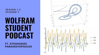
This is a Wolfram Student Podcast episode in which Athanasios Parasivoglos (a Greek mathematics teacher and graduate student) presents his project "Study of the hyperchaotic finance system." He describes a 3-variable (interest rate X, investment demand Y, price exponent Z) dynamical finance model with parameters A (savings), B/β (cost per investment), and γ (elasticity of demand). He implements a numerical solver in the Wolfram Language using the improved Euler method (step size h=0.01) to integrate the ODEs and visualizes results with 3D parametric plots and time-series comparisons. Experiments vary initial conditions (perturbations ~1e-3) and γ; he reports sensitive dependence on initial conditions when γ>1 (chaotic attractor structure) and convergence to a spiral/limit-cycle-like behavior when γ<1 (example γ=0.4). He also discusses pedagogical uses of Wolfram language and future work on PDE projects and mentoring.
Chapters
Hello, everyone, and welcome to a special episode of the Wolfram Student Podcast. I'm Sam.
And I'm Roshan.
And we're your hosts.
This is the Wolfram Student Podcast, where each format we dive into a new innovative project done by high schoolers using the Wolfram language.
For this episode, let's welcome Athanasius, who will be discussing his project on studying hyper chaotic finance systems. Hello, Athanasios.
Good evening, everyone. My name is Athanasios Parasivoglos, and I am from Greece. I am a teacher of mathematics with a proven track record of working in the field of education management. I have a bachelor's degree with an emphasis in mathematics from the University of India, and currently I'm a graduate student in mathematics with specialization in applied mathematics at the Hellenic Open University. My interests are the study and the understanding of partial differential equations. As an undergraduate student, I wrote a thesis entitled the Laplace Equation and the Wave Equation in Plane Spaces. My main goal is to do a PhD on the didactic of differential equation using. Using educational software and in particular, Mathematica. It is an area of mathematics that I have realized that many students struggle with, and I would like to help them make it easier to understand. Cool.
Yeah, that's. That's a perfect intro. And Athanasius is also Wolfram student ambassador, which is another way you've been connected with Wolfram in my mind. So, yeah. Great to have you here.
Yeah, just your graduate studies and partial differential equations are super cool. I like partial differential equations, too. So.
Stuff.
It's nice to meet someone else who so geek about math.
Yeah, yeah, yeah. It's a very interesting area of mathematics, but also a very difficult area of mathematics.
Yeah, for sure. For sure. And just as an icebreaker, what would you say is your favorite voom function? You know, in all the years you've used vu, is there something that sticks in your head?
I haven't thinking about that yet.
Okay. Is there, like, one that's more recent from, like, a project you did?
The recent project I have done, it's about the wave equation with polar coordinates. At my university, it is a project because we study the wave equation with the Schrodinger equation.
Okay, that sounds pretty cool.
Yes. Is a difficult problem because we have, first of all, to prove with the separation of variables, the analytical solution of the wave equation, and then to study this problem for different initial conditions and boundary conditions, and every time the solution changes, they give us other results. Yeah. So cool.
So getting into your project, can you first give us, like, a quick Summary about what it's about.
Yes. This project that we will discuss today is entitled Study of the superhaudic system. The hautic system is a three dimensional hautic system. In this case we will study the haptic final system, a three dimensional holding system. So we rely on a three dimensional holding system with the addition of an extra state, a variable, A dynamic model of finance composed of four sub blocks, production, money, stock and labor force and expressed by three first order different equations. This model describes the time variation of three state variables, the interest rate X, the investment demand Y and the price exponent Z. The chaotic finance system is given as we can see on the screen with these three ordinary differential equations. Every time we will study this problem with given initial conditions and we will solve the particular problem for different value of gamma because this is the point of interest. First of all, we have to define some constants as A we have the savings, B or beta is cost per investment and gamma is the absolute value of the elasticity of demand. These values are given from the paper we studied. The next step we have to define carefully the three differential equations. After we need to use a method that will help us to solve this problem with good accuracy. This problem. In this particular problem we use the improved Euler's method. This technique is an easy extension of Euler method. The improved Euler's method uses an average of the Euler's method and an Euler's method approximation to a given function. This technique requires two functions evaluation instead of one and we use two simple steps of algorithm for implementation. Like every method, this improved Euler method has advantages and disadvantages. The two advantages that this method has it is first, one, it is iterate for the for numerical problems and second, it requires less error than the Euler's method. Hence, for good approximation is obtained with a very small age. It is the step size we use. But of course there is also a disadvantage it is not used for more than third order differential equations. Here we defined, as you can see here, the function Q. We define the improved Euler method. If we want to write the improved Euler method method in Wolfram language, we have to be very careful because it is a big one and a difficult equation. And if we do any mistake it will destroy our project. Now, if we define correct this equation, we plug in the initial conditions for A, B and C as we discussed above and we will use as a step the 0.01 and after that we will see the results on an interval from 0 to 1000. Here we use the parametric 3D plot to see the results of this equation. And we can note that the method give us the characteristic structure of the attractor of the system. We can see that in this 3D animation here. The second case, one of the characteristic of systems with chaotic behavior is also called self sensitive dependence on in nature conditions. So we will change for a small value difference from the beginning in the first initial conditions. And we notice that the new initial conditions differ in each coordinate by 10 at the power of minus 3. As we can see now we are going to study in a smaller interval from 0 to 200 and we use exactly the same code. But the only change that we need to do it is here at the function queue. When we give the initial conditions, we have to change only the initial conditions to our code. As we can see, when we change for the new initial conditions, this program give us a very different plot. Here we can see we have a total different plot than the first one from the first case. When as we can see here. Now the second thing is it is we want to plot these functions the X function, the Y function and the Z function which everyone but everyone of them are dependent on T And here we receive this plot. Now we want to compare the first case and the second case. First of all, we will design the graphic representation of X, Y and P for the first case. Here we receive the following plots for the interval 0 to 200 and we can see there are some differences between of them. Now we will design the graphic representation of X, Y and Z for the modified initial condition for the new initial conditions. As we can see here, the plot it is different than the first case. Let's compare these two solutions on the same plot. Now we use this plot and as we can see from 0 to 60, the the plots are almost identical. But when the T is greater than 60, there are some spot some spots here that the plots are they have big differences. Each of the three plots for X, Y and Z we observe that in the interval 0 to 60 the solution show a slight divergence. The deviation become larger when T is Greater Greater than 0 than 60. Sorry. More specifically, as regards the variables X and Z, we observe larger deviations as we can see in the first case and in the third case. The larger differences are characteristic of so called sensitive dependence on initial conditions. If we try to change again the initial conditions and we use some some bigger numbers, we will observe bigger and differences between the plots. Now we will discuss the other case. When the gamma is less than one, the third Case a case where the gamma the elasticity of demand of the commercials is less than 1. We will study it again on an interval from 0 to 200. We will use again the same code with the same initial conditions. And the only change that we have to do is to choose a number for Gamma less than 1. In this specific case we use for gamma 0.4. This when we use and we run the code, we receive a plot totally different than the above two cases. We notice a big change in the behavior of the system. We can see a spiral trajectory and the system appears converge to a limited circle. We can see see that in the middle of this plot it is totally different from the from the other two plots that we have seen before.
Now.
We want to see if there are any differences if we change a little bit like before the initial conditions. So we choose the initial conditions with a very very small differ at 10 at the 10 of the power of minus 3, like in the second case. And we can see on an interval of from 0 to 1000 the two first plots. They give us the the plots for X, Y and z. For the first case, when we have as initial conditions for x1, for y3 and for z2. And for the second, when we have changed the initial conditions. When we compare these two plots here, we can see that there is no change between these two plots. That means that the system is not sensitive depend is not sensitive dependence on the initial conditions. So the main idea of this project it is that the system is sensitive dependence. When Gamma is greater than one and when we change the initial conditions, the behavior of the system change. And when Gamma is less than 1, we can observe that the system is not sensitive dependence on the initial conditions. For me it was a very interesting problem because I like to study about the economy and finance system. And that gave me a lot of information of what happened in in a hyper hortic dynamic system.
Yeah, this is really cool. I loved your Euler's method to like applying to the partial differential equations and then changing your initial conditions by a little bit. I have a question about your case 3 though. If you look at like the graph that you generated for it, like the interpolating table. Yeah, the purple spiral thing.
Yeah.
No, the thing above that one here. This one?
Yeah, this one.
So that looks totally different from the first two like you said, because the first two had like some kind of similarity I could see. But this one was like completely different.
Except it's completely different.
Right. So but when you like graft when you were like Comparing them further below, they matched up like really nicely in those graphs down there, right?
Yeah. Yes. Here on these plots, we can see as we change the initial conditions, the plot remains exactly the same. They have not.
So you're saying even though, like in this third case, it's different from its graph is different from the first two cases, but when you change its initial conditions, the graphs remain consistent.
So this problem depends on Gamma. If Gamma is greater than 1, we have big changes. If it is less than 1, the changes there are not at all. There are no changes.
So is it. So is the reason that it's consistent here because that function is like a more consistent spiral than the more interesting shape that the first two were?
Exactly.
I see.
Okay. And it is one of the most simple examples because in the initial paper that is published, they study more complex cases. But I have tried to study first the simplest version.
Okay.
Yeah.
Thank you. That looks really interesting.
So thanks a lot for talking about your project. Honestly, it was really cool and I'm glad you were here to share it with us. So if you want to talk for a bit about, you know, your thoughts about the Wolfram language, I'm sure you've used other program languages too. So if you want to compare between them or talk about what's unique about it, if you like something about it, what. What do you think could be different?
I don't know.
And then if you want to talk about your future projects with Wolfram, if you have any in mind, or how you plan to use this in your future education, in your future professional life as a math teacher, perhaps in other ways. Yeah, that's. Go ahead.
Okay. Of course I use Wolfram language for first time in 2013 in my thesis and I was impressed by its capabilities. They cannibally think about this language. It is that even for novice users, it is very easy to learn. There are many books, videos or other documents on Internet that make our life easier. I have never used other language. The first language I used it is Wolfram language and Mathematica. But now also I use Wolfram Alpha. But it helps me to create some problems for my students. And it is very helpful because I give the the. The instructions and the program creates some cool problems for my classes. I'm currently working a project for the wave equation and the Laplace equation in polar coordinates and I will share it on Warframe Community. I have already said some other project on Warframe Community too. In June, I will also be part of Summer cup in Boston as a mentor. And I'm looking forward for this experience. Cool.
Yeah, those are, those sound like wonderful plans and I wish you best of luck with them and you know, I hope you keep doing cool things with worldrum and you know, best of luck in your future endeavors in general too. Perfect.
Yeah.
Thank you very much.
Yeah, it was great to hear from you and your projects and drug goal. So we're looking forward to seeing other projects that you publish. Thank you.
Nice to meet you.
Great to meet you too. Have a wonderful day.
You too.
Have a good day.
Thanks for listening to this episode of the Wolf from Student Podcast. We hope you learned something new and took away insights from today's discussion. If you want to be featured in a future episode, fill out the form@tinyurl.com WSP S2 interest and be sure to.
Tune back in some more time to hear our next episode. Once again, thanks for listening to this episode of the Wolfram Student Podcast.
More from Guy


Cheryl Strauss Einhorn | The Human Edge: Smarter Decisions in the Age of AI | Talks at Google



Rachel Glennerster | Innovation and the Center for Global Development | Talks at Google

Rebecca Winthrop | Rethinking the Purpose of Education in the Age of AI | Talks at Google

Dr. Robert Wachter | A Giant Leap: How AI Is Transforming Healthcare... | Talks at Google



