Wolfram Student Podcast S2 Ep 3: Analyzing River Tributaries and Flood Plains
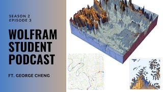
George, a high school senior, extracted river networks from satellite imagery using image processing and morphological methods, then modeled floodplains in 3D by combining elevation data with the Rational Method to estimate peak discharge. He also explored runoff coefficients from satellite color and population-density overlays to assess flood risk.
Chapters
Hello everyone, and welcome to episode three of season two of the Wolfram Student Podcast. I'm Sam.
And I'm Roshan.
And we're your host.
This is the Wolfram Student Podcast where every fortnight we dive into a new innovative project done by high schoolers using the Wolfram language.
For this episode, let's welcome George, who'll be discussing his project on a morphological analysis of river tributaries and floodplains. Hi, George.
Hi, my name is George. I'm a senior at the North Carolina School of Science and Mathematics and I attended the 2023 Wolfram Summer Research.
Cool.
Yeah.
Great to have you here.
And also, I guess, was this the most recent Wolfram research program? Was that your first time experience with Wolfram, or like, have you done some stuff with it before?
Yeah. So before the Wolfram Summer Research Program, I haven't really explored much about the Wolfram language, although I've heard about Steve Wolfram and the many, many cool theories that he came up with. But I've never interacted with the Wolfram language.
Yeah, that's cool. I guess camp's a bit of a learning curve, but at least like, they take time to like, explain everything. So camp is great.
Yeah, of course.
So just a nice, pretty quick question. We like to, you know, just ask people what their favorite Wolfram function is. Do you have any favorites?
Yeah, so my favorite function is listplot3d. I actually use a lot of it in my project. So it's a function that is used to generate a three dimensional plot from a list of data points. And this function was extremely handy for me for visualizing surfaces or terrains as I did a lot of energy and processing. And so basically how it works is that you input a XYZ coordinates and the positions of the matrix will determine the X, y and z points on your morphological graph. And after that it will output a 3D surface plot. And then there's also a lot of options for it. For example, you can use mesh, color function, plot, range, and much, much more.
Yeah, that sounds really cool.
Yeah, Great.
Cool. So do you want to give us like first a quick summary about your project, what it's about, stuff like that?
Yeah, sure. So it's actually really interesting because my project is split into two components. So the first component is, it begins with the analysis of a structure of river tributaries in 2D using Polygon, clustering, satellite imaging, and a cleaning protocols. And then we, we also developed respective tributary tree graphs, morphological graphs and nodes to create a comprehensive tree and 3D model. So this Part of the project was completed actually relatively quickly. So in our second meeting with Stephen Wolfram, I suggested a more profound approach to what I find interesting, which is floods. So afterwards, my second part of the project was examining the morphology, the morphology of floodplains in 3D space, and implementing the rational method, which is one of the oldest frameworks for flood to create relief plots to predict model and visualize flooding elevation. And after that, I created a few more extensions for my project to be more applicable to users around the world.
Anyway, your summary sounded really cool. Do you want to just, I guess, dive straight into your project, explain exactly what all this fancy graphic looks like?
Yeah, sure. So there's actually a few key components. So the first thing that we discovered was something called polygon clustering. So what we did is that we took a Google Maps and then we took all these blue things which are reverse, we characterized it in a derivative and basically extracted all of these components into a single bitmap. And so using this bitmap, we selected and used sorting in order to separate more. We did a lot of cleaning with binarize color negate and dilate and delete small components. Afterwards, we extracted the whole thing using morphological graph. And. And after using morphological graph, there's also this really cool function that you can use called transitive reduction graph. So one of the problems that we had in our project was the cyclic components. And with these cyclic components present, we could not create any trees. And so we have to find a way to remove these cyclic components. And a cool function that we found was transitive reduction graph, which makes all these cyclic components acyclic. And with these cyclic components gone, we are then able to create a tree graph. So this is the end.
Ask a question real quick.
Yeah, sure.
So the cyclic components. So if you could just scroll up a bit. I actually use morphological components in one of my own functions in one of my own projects. This is actually really cool. I think that this is the perfect application for that function. So if you want to scroll up.
A bit and I want to see.
Sort of like the original picture. So you talk about these Oxpro lakes and is that sort of causing the cyclic components?
No, so these are actually. So before the transitive reduction, we actually only just binarized it and then cleaned the data. So when we. Yeah, when we transition the morphological graph to this, to this kind of image, that's when we apply the transitive reduction graph, right?
No, I was just wondering, like, you know that circular thing we see in the morphological graph, what causes that like is it the Oxbow lakes or sort of like basically what's, what's the physical like thing in the river system that's causing the cyclic component to appear that you then obviously remove that with that function, that really interesting function you mentioned. But I'm just curious, so what's causing that initially? That's a difficult.
I think what happens is that these small components that disconnected from the river, when they get dilated, they actually get attached to the river as these very kind of peninsula like structures. And then when we reconnect it back together, it just shows as a cyclic component because sometimes the fitting for the data isn't as accurate as we hoped. And so that's when we have to reapply the acyclic to get rid of that small little blotch.
Got it. Yeah, that makes sense. Cool.
And so another part of the first part of the project is mapping river branches on maps. And so while we did evaluate polygons, extracting polygons across a multitude of different maps with a lot of color schemes is not trivial. And so we use the functions nearest and color replace to make the association of the rivers blue to our desired blue color. And so this takes the variability out of the colors that we have to extract and makes it a lot easier for us because we don't have to account for every single color and instead match the nearest blue to our blue for when we're extracting our morphological components. And so here is a large function that we coded to create this, this image which shows the different branch splits. So I can walk you guys through the code. So first thing that we did is that we took the map of Paris, which is one of our various, one of our model cities. So what we first did is that we took a geographics and took everything into a vector. And so by using a vector we're able to create everything into polygons. And after that we separate the raw layers using Geo2 graphics layer. And then we set our watercolor function. So as I mentioned earlier, the watercolor function is to make different shades of blue the same blue. And then we applied the river branch map, which is basically to resize every single map onto a 10 by 10 mile satellite image. And then we did a river branch map function which is basically to take all of these components, extract them, overlay them on the Paris map, as well as dwell more into the small components like morphological tree graphs, see the splits, plot the points on these splits and overlay it on the entire Paris map. 2. So this whole code basically the purpose of it is to identify the splits inside the streams through a function called stream splits, and being able to map this back on the river and back on the map once again. So while this may seem like intimidating code, it's a lot of repeats. And I think if we cleaned it better, we could have made it a lot less intimidating. And then using this code, we actually applied it and tested on simple river systems. So simple river systems might be very overlooked because you might think that if the river is simple, then it would be easier for us to apply these functions. However, sometimes the simple ones are the hard ones, because these simple river systems have a lot of small components, minute components, that are not trivial. And so if these components get jumbled together and make a incorrect river, that is a problem too. And so what we delved into was a model example from Jackson, Mississippi. And so again, we apply the polygon components function in which we use select and cases to isolate the river apart from other small components. After doing this, we again use binarization. As I mentioned earlier, we used the functions binarize and flatten and took this whole river and made it into a binary map. And after that, we did a lot more cleaning, including delete small, small components to make one simple river. And then that's when I started delving into to see if there's more accurate representations of this river other than morphological graphs. So I created a morphological graph and compared it with the 3D reduction graph. I also compared it with the tree graph. And so some common flaws that we saw with this type of approach is that we saw that minor tributaries, so even those that are only visible, like let's say only 1% of the river, was shown in full in the tree graph. Because the tree graph cannot differentiate between a large tributary and a small tributary, it was extremely hard for us to scale how big the tributaries, the individual tributaries are. And so one of the solutions to that was to use something called stream order, which is something I'll dive into later on in my presentation. And so with that flaw in mind, we moved on into complex river systems. So complex river systems have the same problem as simple river systems. Complex river systems have components and tributaries that are overlooked rather than underlooked. And so we examined a model example from Alaska. So, repeating the same steps, I'm just going to skip to the end. We found a morphological graph that is partially representative of the of the rivers that we saw in Alaska. So one of the large, like one of the main components, one of the main flaws that we saw in this was that it generally it did not account for large parts of the river, and it also count multiple. It also counted large bodies of water as multiple rivers. And one way around that is to increase the dilation. However, when we increase the dilation for one type of river, it will ruin other types of rivers, like simple river systems. And so in the end, what we decided to do is that we decided to calibrate it based on how dense the water is. And so if the water is over a certain threshold, then it will refer to the complex river system code. And if it's under a certain threshold or refer to a simple river system code. And so with all of this, I presented it to Stephen Wolfram, and he was pretty happy that I was able to differentiate river tributaries just from a map. And so this is actually supposed to be my quote unquote project for the Wolfram Summer Research Program. But because I finished it pretty early, with a lot of time in hand, I moved on to the second part of my project, which is a, I would say a more interesting dive into floods. And so I guess one of the. I guess I'll start with a summary of why I did floods. So I used to live in the south, so I was born in Georgia. And every single year I remember a hurricane will come through or some natural disaster and a lot of homes are swept off. Especially I think it was like 2013, 2014, it was a lot of natural disasters. And so I wanted to see if there was a better way to predict floods based on terrain data. So rather than using satellite data and ignoring the elevation planes, I actually incorporated the elevations, the permeability, as well as real time information in order to analyze floods. So currently there are also no built in functions to vertical floods. And so that incorporating this would, I guess, serve as a proof of concept for a future development of flood frameworks in Mathematica. So the specific framework I use is something called Q equals CIA or the rational method. So using the rational method, we are able to account for three variables. The C, the permeability of the surface, I, the intensity of the rainfall, and A, the acres of land it was on to create Q, which is the total stream rise elevation during the flood. So in order to do this, I first swelled into imaging processing. So image processing is something that I feel like often underlooked in Mathematica. So a lot, I think, I think a lot of projects dwell more into the numerical analytical side of Mathematica, but I feel like Mathematica also has a lot of uses, especially in image processing. So the first step of this section is to find a way to take satellite imagery of a geographic location using a function called geoimage and then extracting the river basin using imaging processing like image compose and my favorite function, lispod3d. And so for this part of the project I used the model City Juno to model a lot of my satellite images, terrain data, etc. So I'll just start by introducing some of the important functions that you may or may not have recognized from my previous section. So one of the most important functions functions was GEO Image. So GEO Image, Color Negate, Binarize and Image recolor. All four of these functions basically takes a satellite image, extracts the river from it by ignoring all the other images, recoloring the color because I thought black was a little ugly, and then putting it back onto the satellite image using the image compose function. And so how exactly I did this was pretty simple really by using Mathematica's options. So in Mathematica there after like the, I guess the main part of the function there are the options part which is basically I guess add ons. So if you think about it in like a more real world, real world example, you get a sports car but you add, you can add a lot of attachments on it. And so what we first did was that we overlaid satellite image and river image and then we used Lispod3D to plot it in a 3D image. And so Lispot3D took the geo elevation data of Juno, Alaska. Then it took the geo range which is the 10 by 10 mile around Alaska, used the mesh function to I guess make the, make the peaks more stand out and also to have these round surfaces. And I plotted all of the data and through plotting all of the data also set the texture into the satellite image so it doesn't look black and white. Then I just filling on the bottom so it doesn't look hollow. And I put the filling style as opacity one so that doesn't look clear. And the image size I set to 1000. Okay, so I'm going to move on to relief plots. So again, if you recall from my first explanation of polygon extraction, I used it again. And so by extracting this color, which is the omnipresent color, I guess in Google Maps I use color replace to fill in the quote unquote flooded space. And I use a dynamic app module to synchronize the reflective changes made. And so through this animation, which I unfortunately had to take out because it was exceeding the max File limit uploaded to the warfare community, you can actually manipulate the rainfall data in order to get a set relief plot that you're going to use and transpose onto a 3D data. And so how I did it was that let's take Juno again. I took the geo elevation data of Juno and I projected it automatically and used and specified the imperial imperial units. And then after that I create a side function here which is basically to define my variables of the minimum elevation and the maximum elevation. This is so that the cities outside of Juno can also use this data. Because if we were to hard code everything, then we're going to have to hard code Juno data and we're going to have to hard code the minimum elevation data of only Juno and the maximum elevation of only Juno as well. And so this is basically some, I think, ease for transition if we're going to transition it to a more applicable cities. And so after that I used again manipulate data which is where you see this bar from to manipulate the rainfall to serve as a proof of concept. And then I put this options as synchronized updating. True. This is so that the dynamic app module can, which you, which you see here, the Juno relief plot can reflect this data to synchronize onto a map. And so by, and so after you see the flooded space by using this map, you can plot it on a Lispot 3D. And so what's different from this Lispot 3D versus let's say a satellite Lisp 3D is that you can actually see where it's flooded. So it will automatically exclude the areas that's not flooded and only include the relief plot area where it has been flooded. And so if I zoom in a little bit, you can actually see that there are the clear components in which the mountains are not flooded and there are components much lower that are flooded. And so we thought that was a pretty cool application and a pretty good segue into creating our actual mathematical function, which is Q equals CIA. So I'll give you a quick introduction of what Q equals CIA is, its introduction and its usages. And so mainly the rational method, or TCIA is used for determining peak discharge. And so this method is traditionally used to basically provide an estimate on storm sewers, channels and other stormwater structures, especially in urban areas as well as rural and suburban areas. And so what's interesting about this is that as I mentioned earlier, there are three components. So the first component, the C component, is basically the coefficients, the runoff coefficients for the rational formula. And so basically there was, I think around 30, 20, 30 parameters based on the environment and how permeable the soil is. And so based on these coefficients, we were able to gauge how much water actually seeps into the ground and how much goes on inside the city or in on unpermeable surfaces could lead to flash flooding. And so by using this data, we actually had to build something really interesting. So that's when we extracted other colors from Google Maps. And so instead of only extracting this blue color, we actually had to extract all of the possible colors, which is eight from satellite, from a Google map image and portray and set a associate with all of these colors towards these permeable coefficients. And so when we did that, we can thread this and basically take the keys of all of this, of the colors that were defined and set a weight. So what we did with the weight was that it took the color density. So let's suppose it was in a very urban area. The color density of this gray color would be far more than, let's say a color density of this green color, which represented trees. And so because the gray color had a higher coefficient runoff, we multiplied this number by the percentage of the color present in the satellite map. This will essentially give us a weighted mean. And so by using this weighted mean, we took the weighted mean and averaged it to create the, to create the city weight by color function. And so with our city weight by color function and averaging all these weighted means, we're able to create a finite runoff coefficient for the entire city area map. So this was like an innovative, this was an innovative way to tackle to use Google Maps in order to create a runoff coefficient for a particular city area. Of course there are more accurate ways, but it will require much more data. It will probably require data like us from the National Ocean Ocean like the noaa, and a lot more real time data as well. And so with our I calculation was the intensity. And so the intensity was quite easy to calibrate. So what we did was that we took the weather data over the past 20 years of a specific area through the weather data function. It was in Mathematica. And we're able to find the average annual rainfall measurement in centimeters, which we converted to inches. And then we mapped the intensity of rainfall instead of proportional to how high that annual rainfall is, using a which function. So this is one of the most basic functions, I think, inside the whole code, which is which is basically taking all this data, setting different parameters for the which function and calibrating the intensity. And lastly, for the irrational method, we did the a Calculation, which is the acres very self explanatory, 20 miles squared is equal to 256,000 acres. And so we apply this, we combine everything to get a final number for Juno. So what does this actually mean? So this means that there's roughly 1422 cubic feet per hour for a flash flood event in Juneau, Alaska. And so by using this data we can again take what we know, which is a relief calculation and integration plot analysis that we did earlier, incorporate the number that we got from our junot total river increase and finally plot it all into this lispot3d function. So this lispot3d I guess is the culmination of the second part of my project, which is basically to implement everything we know about relief plots with one additional tweak from genototal river increase here. So the pod 3D range will then show a extra layer I guess in a sort ranging from the minimum increase to the minimum increase plus the total river increase that we found from our rational method. Again we tested on simple river systems, the same one from Jackson we saw. So all of this might seem a lot more menacing than it is, but it's just a lot of repeats. And if we cleaned it it would probably been around three lines. But in the end we saw in a flash flood events for Jackson, Mississippi, it will rise quite far. And again we did another complex river last river analysis system, this time again in Anchorage. And we saw that if the flush valve was to occur in Anchorage, it wouldn't be affecting as well. This actually made a lot of sense considering that Anchorage is very dry and does not receive a lot of precipitation, whereas Jackson, Mississippi does release does receive a lot of precipitation as well. And so I guess at the very end we just try to tie everything together using what we know from our stream orders and put overlaying the stream order onto our floodplain to create a cool graphic like this. And again, as I mentioned earlier, we did do a few extensions. So one of the extensions was a populated relation density model to see which areas will be the most affected by this flood. Again this code is a lot more menacing, but basically what we did is that we created a which function in order to calculate for the texture density which correlates to color. And the color will be keyed in onto a combined image, which is an overlay basically. And lastly, the last interesting thing I would like to talk about is a large scale modeling. And so basically this takes the certain width of certain rivers and tributaries and determines the length of notable bridges across the River. And so this can basically, I guess, model where floods are like flood blank. Flood banks are most likely to get destroyed in a case of flash floods because it shows where the river is the widest and where it's most likely to be breached are the white dots because that's where the rivers are the most narrow. And in conclusion. So again to reiterate in conclusion, my project first established a framework for detecting river tributaries which is very interesting because rivers are actually not entity geo entities in Mathematica, they're only entities. And so being able to extract this geographic data from rivers is something pretty novel. And we also establish nodes and river terpitator branches, created trees for tributaries for finally combining everything together for a floodplain analysis in which we examine geographic elevation data using a specific framework called QCIA before finally analyzing population density and creating pure anonymous functions to generalize all geographic locations. Lastly, we combined our two findings to create a comprehensive 3D model that models both are river tributary splits and floodplains. Yeah.
Yeah, that looks really cool. Thank you for your.
Yeah, that was, I mean, your explanation.
Was really, really helpful for, you know.
I'm sure anyone who's trying to understand this. It can be kind of tricky at first glance to understand why everything's being.
Manipulated in the way it is or.
So what the steps are. Especially because, you know, and I'm sure you know this, but like a lot of, you know, a lot of projects done on a tight timeline like this are maybe, you know, they don't have the cleanest code because that takes like extra effort. And when you're just like watching things together and making it work, which is, which did happen to me at camp a fair bit when I did that two years ago. So yeah, doing that, that definitely. So it helps to just have an explanation of the. So thanks for that.
Yeah, thank you. Yeah. Sam. Yeah.
So really cool to see everything you've done with this. So I guess I'm just curious, do you have any future steps for like how you want to take this project specifically? Maybe other work with Wolfram language?
Yeah, so actually a very challenging part of this project was examining straw or stream order. So that was what I spent three days on. Straw. Stream order basically classifies and ranks rivers and streams based on the branching. And so it was introduced in 1950s to better characterize rivers. And so it will follow first order, second order, third order in which smaller tributaries would join to form bigger tributaries. And so these tributaries, if you're going to do an iterative step, is actually extremely hard to identify because you're going to have to tell the program to recalculate every single time there's a new tributary. It's also very time intensive too, and so that's probably something I would like to work on more in this project. But I think outside I'm probably thinking of working a lot with chemistry because I really like chemistry and seeing all these really cool functions with chemistry and Wolfram being its nature, being allowed to real world data directly into our computations is really exciting.
I feel like, yeah, that's really cool. Chemistry is different, definitely interesting and it's like, I guess a bit of a change from our current project. But yeah. Okay. Thank you so much for coming on and, you know, sharing your project with us and all your really great explanations about how all of this works because I've definitely learned a lot.
Thank you too.
Thank you.
Thanks for listening to this episode of.
The Wolfram Student Podcast.
We hope you learned something new and took away insights from today's discussion. If you want to be featured in a future episode, fill out the form@tinyurl.com WSP S2 interest and be sure to.
Tune back in two weeks time to hear our next episode. Once again, thank you for listening to this episode of Oops. Wolfram Student Podcast.
More from Guy


Cheryl Strauss Einhorn | The Human Edge: Smarter Decisions in the Age of AI | Talks at Google



Rachel Glennerster | Innovation and the Center for Global Development | Talks at Google

Rebecca Winthrop | Rethinking the Purpose of Education in the Age of AI | Talks at Google

Dr. Robert Wachter | A Giant Leap: How AI Is Transforming Healthcare... | Talks at Google



